Spectroscopy principles
410 likes | 720 Views
Spectroscopy principles. Jeremy Allington-Smith University of Durham. Contents. Reflection gratings in low order Spectral resolution Slit width issues Grisms Volume Phase Holographic gratings Immersion Echelles Prisms Predicting efficiency (semi-empirical). Generic spectrograph layout.

Spectroscopy principles
E N D
Presentation Transcript
Spectroscopy principles Jeremy Allington-Smith University of Durham
Contents • Reflection gratings in low order • Spectral resolution • Slit width issues • Grisms • Volume Phase Holographic gratings • Immersion • Echelles • Prisms • Predicting efficiency(semi-empirical)
Generic spectrograph layout Camera Collimator Focal ratios defined as Fi = fi / Di
Grating equation n1 n2 A B b a A’ B’ a • Interference condition: path difference between AB and A'B' • Grating equation: • Dispersion: f2 dx db
"Spectral resolution" dl l • Terminology (sometimes vague!) • Wavelength resolutiondl • Resolving power • Classically, in the diffraction limit, Resolving power = total number of rulings x spectral order I.e. • But in most practical cases for astronomy (c < l/DT), the resolving power is determined by the width of the slit, so R < R* Total grating length
Spectral resolution • Spectral resolution: • Projected slit width: Conservation of Etendue(nAW) Image of slit on detector Camera focal length
Resolving power Size of spectrograph must scale with telescope size • Illuminated grating length: • Spectral resolution (width) • Resolving power: • expressed in laboratory terms • expressed in astronomical terms since and Collimator focal ratio Physical slitwidth Grating length Angular slitwidth Telescope size
Importance of slit width • Width of slit determines: • Resolving power(R)since Rc = constant • Throughput (h) • Hence there is always a tradeoff between throughput and spectral information • Functionh(c) depends on Point Spread Function (PSF) and profile of extended source • generally h(c) increases slower than c+1whereas R c-1 so hR maximised at small c • Signal/noise also depends on slit width • throughput ( signal) • wider slit admits more sky background ( noise)
Signal/noise vs slit width • For GTC/EMIR in K-band (Balcells et al. 2001) SNR falls as slit includes more sky background Optimum slit width
Anamorphism dispersion Output angle • Beam size in dispersion direction: • Beam size in spatial direction: • Anamorphic factor: • Ratio of magnifications: • if b < a, A > 1, beam expands • W increases R increases • image of slit thinner oversampling worse • if b > a, A < 1, beam squashed • W reduces R reduces • image of slit wider oversampling better • if b = a, A = 1, beam round • Littrow configuration Input angle
Generic spectrograph layout Camera Collimator Fi = fi / Di
Blazing b = active width of ruling (b a) • Diffracted intensity: • Shift envelope peak to m=1 • Blaze condition specular reflection off grooves: also since Interference pattern Single slit diffraction F = phase difference between adjacent rulings q = phase difference from centre of one ruling to its edge
Efficiency vs wavelength • Approximation valid for a > l • lmax(m) = lB(m=1)/m • Rule-of-thumb: 40.5% x peak at (large m) • Sum over all orders < 1 • reduction in efficiency with increasing order 2 3 4 5 6 (See: Schroeder, Astronomical Optics)
Order overlaps Effective passband in 1st order Don't forget higher orders! Intensity 1st order blaze profile m=1 First and second orders overlap! m=2 Passband in 2nd order Zero order matters for MOS 2nd order blaze profile Passband in zero order m=0 Wavelength in first order marking position on detector in dispersion direction (if dispersion ~linear) 1st order 0 lL lC 2lL lU 2lU (2nd order) 0 lL lU
Order overlaps dispersion Detector 1st order To eliminate overlap between 1st and 2nd order • Limit wavelength range incident on detector using passband filter or longpass ("order rejection") filter acting with long-wavelength cutoff of optics or detector (e.g. 1100nm for CCD) • Optimum wavelength range is 1 octave (then 2lL = lU) • Zero order may be a problem in multiobject spectroscopy Zero order 2nd order
Predicting efficiency • Scalar theory approximate • optical coating has large and unpredictable effects • grating anomalies not predicted • Strong polarisation effect at high ruling density (problem if source polarised or for spectropolarimetry) • Fabricator's data may only apply to Littrow (Y = 0) • convert by multiplying wavelength by cos(Y/2) • grating anomalies not predicted • Coating may affect grating properties in complex way for largeg (don't scale just by reflectivity!) • Two prediction software tools on market • differential • integral
GMOS optical system CCD mosaic (6144x4608) Mask field (5.5'x5.5') Detector (CCD mosaic) Science fold mirror field (7') Masks and Integral Field Unit From telescope
Example of performance • GMOS grating set • D1 = 100mm, Y = 50 • DT = 8m,c = 0.5" • m = 1, 13.5mm/px • Intended to overcoat all with silver • Didn't work for those with large groove angle - why? • Actual blaze curves differed from scalar theory predictions
Grisms • Transmission grating attached to prism • Allows in-line optical train: • simpler to engineer • quasi-Littrow configuration - no variable anamorphism • Inefficient for r > 600/mm due to groove shadowing and other effects
Grism equations • Modified grating equation: • Undeviated condition: n'= 1,b = -a = f • Blaze condition: q=0lB = lU • Resolving power (same procedure as for grating) q = phase difference from centre of one ruling to its edge
Volume Phase Holographic gratings • So far we have considered surface relief gratings • An alternative is VPH in which refractive index varies harmonically throughout the body of the grating: • Don't confuse with 'holographic' gratings (SR) • Advantages: • Higher peak efficiency than SR • Possibility of very large size with highr • Blaze condition can be altered (tuned) • Encapsulation in flat glass makes more robust • Disadvantages • Tuning of blaze requires bendable spectrograph! • Issues of wavefront errors and cryogenic use
VPH configurations • Fringes = planes of constant n • Body of grating made from Dichromated Gelatine (DCG) which permanently adopts fringe pattern generated holographically • Fringe orientation allows operation in transmission or reflection
VPH equations • Modified grating equation: • Blaze condition: = Bragg diffraction • Resolving power: • Tune blaze condition by tilting grating (a) • Collimator-camera angle must also change by 2a mechanical complexity
VPH efficiency Barden et al. PASP 112, 809 (2000) • Kogelnik's analysis when: • Bragg condition when: • Bragg envelopes (efficiency FWHM): • in wavelength: • in angle: • Broad blaze requires • thin DCG • large index amplitude • Superblaze
VPH 'grism' = vrism • Remove bent geometry, allow in-line optical layout • Use prisms to bend input and output beams while generating required Bragg condition
Limits to resolving power • Resolving power can increase as m, r and W increase for a given wavelength, slit and telescope • Limit depends on geometrical factors only - increasing r or m will not help! • In practice, the limit is when the output beam overfills the camera: • W is actually the length of the intersection between beam and grating plane - not the actual grating length • R will increase even if grating overfilled until diffraction-limited regime is entered (l > cDT) Grating parameters Geometrical factors
Limits with normal gratings • For GMOS with c= 0.5", DT= 8m,D1 =100mm, Y=50 • Rand l plotted as function of a • A(max) = 1.5 since D2(max) = 150mmR(max) ~ 5000 Normal SR gratings Simultaneous l range
Immersed gratings • Beat the limit using a prism to squash the output beam before it enters the camera: D2 kept small while W can be large • Prism is immersed to prism using an optical couplant (similar n to prism and high transmission) • For GMOS R(max)~ doubled! • Potential drawbacks: • loss of efficiency • ghost images • but Lee & Allington-Smith (MNRAS, 312, 57, 2000) show this is not the case
Limits with immersed gratings • For GMOS with c= 0.5", DT= 8m,D1 = 100mm • R and l plotted as function of a • With immersion R ~ 10000 okay with wide slit Immersed gratings
Echelle gratings • Obtain very high R(> 105) using very long grating • In Littrow: • Maximising g requires large mr since mrl= 2sing • Instead of increasing r, increase m • Echelle is a coarse grating with large groove angle • R parameter = tang (e.g R2 g= 63.5) Groove angle
Multiple orders • Many orders to cover desired ll: Free spectral range Dl = l/m • Orders lie on top of each other: l(m) =l(n) (n/m) • Solution: • use narrow passband filter to isolate one order at a time • cross-disperse to fill detector with many orders at once Cross dispersion may use prisms or low dispersion grating
Echellette example - ESI Sheinis et al. PASP 114, 851 (2002)
Prisms • Useful where only low resolving power is required • Advantages: • simple - no rulings! (but glass must be of high quality) • multiple-order overlap not a problem - only one order! • Disadvantages: • high resolving power not possible • resolving power/resolution can vary strongly with l
Dispersion for prisms • Fermat's principle: • Dispersion:
Resolving power for prisms Angular width of resolution element on detector • Basic definitions: • Conservation of Etendue: • Result: • Comparison of grating and prism: Angular dispersion Angular slitwidth Beam size Telescope aperture Disperser 'length' 'Ruling density'
Prism example A design for Near-infrared spectrograph* of NGST • DT = 8m, c= 0.1", D1 = D2 = 86mm, 1 <l< 5mm • R 100 required Raw refractive index data for sapphire Collimator Slit plane Double-pass prism+mirror Detector Camera * ESO/LAM/Durham/Astrium et al. for ESA
Prism example (contd) • Required prism thickness,t: • sapphire: 20mm • ZnS/ZnSe: 15mm • Uniformity in dl orR required? • For ZnS: n2.26 a=75.3 f= 12.9
Appendix: Semi-empirical efficiency prediction for classical gratings
Efficiency - semi-empirical • Efficiency as a function of rl depends mostly on g • Different behaviour depends on polarisation: P - parallel to grooves (TE) S - perpendicular to grooves (TM) • Overall peak at rl = 2sing (for Littrow examples) • Anomalies (passoff) when light diffracted from an order at b = p/2 light redistributed into other orders • discontinuities at (Littrow only) • Littrow: symmetry m 1-m • Otherwise: no symmetry (rl depends on m,Y) double anomalies • Also resonance anomalies - harder to predict
Efficiency - semi-empirical (contd) Different regimes for blazed (triangular) grooves g < 5 obeys scalar theory, little polarisation effect (P S) 5 <g < 10S anomaly at rl 2/3, P peaks at lowerrl than S 10 < g < 18various S anomalies 18 < g < 22anomalies suppressed, S >> P at large rl 22 < g < 38strong S anomaly at P peak, S constant at large rl g > 38S and P peaks very different, efficient in Littrow only NOTE Results apply to Littrow only From: Diffraction Grating Handbook, C. Palmer, Thermo RGL, (www.gratinglab.com) rl a=b