Converting formulas into a normal form
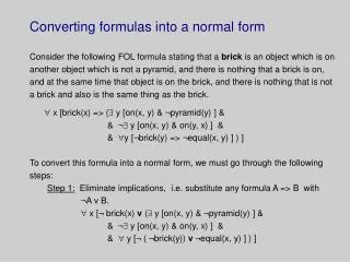
Converting formulas into a normal form. Consider the following FOL formula stating that a brick is an object which is on another object which is not a pyramid, and there is nothing that a brick is on, and at the same time that object is on the brick, and there is nothing that is not

Converting formulas into a normal form
E N D
Presentation Transcript
Converting formulas into a normal form Consider the following FOL formula stating that a brick is an object which is on another object which is not a pyramid, and there is nothing that a brick is on, and at the same time that object is on the brick, and there is nothing that is not a brick and also is the same thing as the brick. x [brick(x) => ( y [on(x, y) & ¬pyramid(y) ] & & ¬ y [on(x, y) & on(y, x) ] & & y [¬brick(y) => ¬equal(x, y) ] ) ] To convert this formula into a normal form, we must go through the following steps: Step 1: Eliminate implications, i.e. substitute any formula A => B with ¬A v B. x [¬ brick(x) v ( y [on(x, y) & ¬pyramid(y) ] & & ¬ y [on(x, y) & on(y, x) ] & & y [¬ ( ¬brick(y)) v ¬equal(x, y) ] ) ]
Converting formulas into a normal form (cont.) Step 2: Move negations down to atomic formulas. This step requires the following transformations: ¬ (A v B) ¬A & ¬B ¬ (A & B) ¬A v ¬B ¬ ¬A A ¬ x A(x) x (¬ A(x)) ¬ x A(x) x (¬ A(x)) x [¬ brick(x) v ( y [on(x, y) & ¬pyramid(y) ] & & y [¬ on(x, y) v ¬ on(y, x) ] & & y [brick(y) v¬equal(x, y) ] ) ]
Converting formulas into a normal form (cont.) Step 3: Eliminate existential quantifiers. Here, the only existential quantifier belongs to the sub-formula y [on(x, y) & ¬pyramid(y) ]. This formula says, that given some x, we can find a function that takes x as an input, and returns y. Let us call this function support(x). Functions that eliminate the need for existential quantifiers are called Skolem functions.Here support(x) is a Skolem function. Note that the universal quantifiers determine the arguments of Skolem functions: there must be one argument for each universally quantified variable whose scope contains the Skolem function. x [¬ brick(x) v ( on(x, support(x)) & ¬pyramid(support(x)) ) & & y [¬ on(x, y) v ¬ on(y, x) ] & & y [brick(y) v ¬equal(x, y) ] ) ]
Converting formulas into a normal form (cont.) Step 4: Rename variables, if necessary, so that no two variables are the same. x [¬ brick(x) v ( on(x, support(x)) & ¬pyramid(support(x)) ) & & y [¬ on(x, y) v ¬ on(y, x) ] & & z [brick(z) v ¬equal(x, z) ] ) ] Step 5: Move the universal quantifiers to the left. x y z [¬ brick(x) v ( on(x, support(x)) & ¬pyramid(support(x)) ) & & [¬ on(x, y) v ¬ on(y, x) ] & & [brick(z) v ¬equal(x, z) ] ) ]
Converting formulas into a normal form (cont.) Step 6: Move disjunctions down to literals. This requires the following transformation: A v (B & C & D) (A v B) & (A v C) & (A v D) x y z [ ( ¬ brick(x) v on(x, support(x))) & & ( ¬ brick(x) v ¬pyramid(support(x)) ) & & [¬ brick(x) v ¬ on(x, y) v ¬ on(y, x) ] & & [¬ brick(x) v brick(z) v ¬equal(x, z) ] ) ] Step 7: Eliminate the conjunctions, i.e. each part of the conjunction becomes a separate axiom. x ( ¬ brick(x) v on(x, support(x))) x( ¬ brick(x) v ¬pyramid(support(x)) ) x y [¬ brick(x) v ¬ on(x, y) v ¬ on(y, x) ] x z [¬ brick(x) v brick(z) v ¬equal(x, z) ] ) ]
Converting formulas into a normal form (cont.) Step 8: Rename all the variables so that no two variables are the same. x ( ¬ brick(x) v on(x, support(x))) w( ¬ brick(w) v ¬pyramid(support(w)) ) u y [¬ brick(u) v ¬ on(u, y) v ¬ on(y, u) ] v z [¬ brick(v) v brick(z) v ¬equal(v, z) ] ) ] Step 9: Eliminate the universal quantifiers . Note that this is possible because all variables now are universally quantified, therefore the quantifiers can be ignored. ¬ brick(x) v on(x, support(x)) ¬ brick(w) v ¬pyramid(support(w)) ¬ brick(u) v ¬ on(u, y) v ¬ on(y, u) ¬ brick(v) v brick(z) v ¬equal(v, z)
Converting formulas into a normal form (cont.) Step 10 (optional): Convert disjunctions back to implications if you use the “implication” form of the resolution rule. This requires the following transformation: (¬A v ¬B v C v D) ((A & B) => (C v D)) brick(x) => on(x, support(x)) brick(w) & pyramid(support(w)) => False brick(u) & on(u, y) & on(y, u) => False brick(v) & equal(v, z) => brick(z)
Converting formulas into a normal form: summary The procedure for translating FOL sentences into a normal form is carried out as follows: • Eliminate all of the implications. • Move the negation down to the atomic formulas. • Eliminate all existential quantifiers. • Rename variables • Move the universal quantifiers to the left. • Move the disjunctions down to literals • Eliminate the conjunctions • Rename the variables • Eliminate the universal quantifiers. • (Optional) Convert disjunctions back to implications.
Logical reasoning systems Recall that the two most important characteristics of AI agents are: • Clear separation between the agent’s knowledge and inference engine. • High degree of modularity of the agent’s knowledge. We have already seen how these features are utilized in forward and backward chaining programs (these are referred to as production systems). Next, we discuss three different implementations of AI agents based on the same ideas, namely: • AI agents utilizing logic programming (typically implemented in a PROLOG-like language). • AI agents utilizing frame representation languages or semantic networks. • AI agents utilizing description (or terminological) logics.
Logic programming and Prolog. Consider a knowledge base containing only Horn formulas, and a backward chaining program where all of the inferences are performed along a given path until a dead end is encountered (i.e. the underlying control strategy is depth- first search); when a dead end is encountered, the program backs up to the most recent step which has an alternative continuation. Example: Let the KB contain the following statements represented as PROLOG clauses (next to each clause, a LISP-based implementation is given). mammal(bozo). (remember-assertion ‘(Bozo is a mammal)) mammal(Animal) :- hair(Animal). (remember-rule ‘(identify1 ((? animal) has hair) ((? animal) is a mammal))) ?- mammal(deedee). (backward-chain ‘(Deedee is a mammal)) ?- mammal(X). (backward-chain ‘((? X) is a mammal)) Note that PROLOG uses a prefix notation, variables start with uppercase letters, and constants are in a lowercase. Each statement ends with a period.
PROLOG syntax If a rule has more than one premise, a comma is used to separate the premises, i.e. A & B & C & D => H is written in PROLOG as H :- A, B, C, D. head body Rule of the form A v B v C v D => H can be presented as follows: H :- A; B; C; D. Note that this is equivalent to H :- A. H :- B. H :- C. H :- D. To represent negated antecedents, PROLOG uses the nagation as failure operator, i.e. A & ¬B => H is represented in PROLOG as H :- A, not(B).
The negation as failure operator Note that notis not a logical negation. This operator works as follows: to satisfy not(B), PROLOG tries to prove B; if it fails to prove B, not(B) is considered proved. The negation as failure operator is based on the so-called closed-world assumption. This states that if a theorem were true, then an axiom would exist stating it as being true. If such an axiom does not exist, we can assume that the theorem is false. The closed-world assumption is very dangerous, because it may introduce inconsistencies in the KB. Example: Assume not(B) is found true. Next assume that B is entered as an axiom. Now, the KB contains both, B and not(B).
Managing assumptions and retractions Consider the following PROLOG program: D :- not(A), B. D :- not(C). Rules F :- E, H. N :- D, F. E. Premises H. ?- N. Query To prove N, Prolog searches for a rule, whose head is N. Here N :- D, F. is such a rule. For this rule to fire, D and F must be proven in turn: • To prove D, consider rule D :- not(A), B. fails, because of B. • To prove D, consider rule D :- not(C). succeeds. • F can be easily proved, because E and H are declared as premises Therefore, N is proved (based on the fact that E and H are true, and assuming that C is false).
Example (cont.) Assume now that the system learns C. What happens to D and N, respectively? Obviously, D and N must be retracted. The BIG question is how to dothis. Note that there are other reasons for which we may want to retract a sentence, such as: • To make the system “forget”. • To update the current model of the world. PROLOG does not have means for implementing retractions, that is it can only handle incomplete knowledge, but not inconsistent knowledge.
Note the difference between retracting a sentence and adding the negation of that sentence. In our example, if not(C) is retracted, the system will not be able to infer either C, or ¬C. Whereas, if ¬C KB and we add C, then the system can infer both C and ¬C. The process of keeping track of which additional statements must be retracted when we retract not(C) (D and N in our example) is called truth maintenance. Although PROLOG cannot do retractions, it is a non-monotonic system, because it allows inferences to be made from incomplete information (thanks to the negation as failure operator).
Generation of explanations The ability to explain its reasoning is one of the most important features of KBS. There are different ways to do that: • To record the reasoning process, and keep track of the data upon which the conclusion depends. • To keep track of the sources of each data item, for example “provided by the user”, “inferred by rule xx”, etc. • To keep a special note as part of the rule that contains an explanation. Example: Given the following rules H & B => Y, C => B, ¬C => ¬B, A => X & Y, C => D, ¬A => C. Given that H is true, prove Y. Explanation1Explanation 2 Y is a conclusion of rule H & B => Y, Y because A is unknown (meaning and premises B and H (how B was that by the negation as failure rule proved is not relevant for the we can assume ¬A) and H is true. explanation of Y). Or, Y because of H until ¬A.
Reasoning with incomplete knowledge: default reasoning (AIMA, page 459) Consider the conditions under which Y is true in the above example: for Y to be true, H must be true and it must be reasonable to assume ¬A. This can be represented by means of the following rule: H : ¬A Rules of this type are called default rules. Y The general form of default rules is: A : B1, B2, … , Bn C where: A, B1, B2, … , Bn, C are FOL sentences; A is called the prerequisite of the default rule; B1, B2, … , Bn are called justifications of the default rule; C is called the consequent of the default rule.
Example Let Tweety be a bird, and because we know that birds fly we want to be able to conclude that Tweety flies. Bird(Tweety) Bird(X): Flies(X) This rule says “If X is a bird, and it is consistent to Flies(X) believe that X flies, then X flies”. Given only this information about Tweety, we can infer Flies(Tweety). Assume that we learn Penguin(Tweety). Because penguins do not fly, we must have the following rule in the KB to handle penquines: Penguin(X): ¬Flies(X) ¬Flies(X) We can infer now Flies(Tweety) (according to the first rule), and ¬Flies(Tweety) according to the second rule. To resolve this contradiction, we may want to always prefer the “more specific rule”, which in this case will first derive ¬Flies(Tweety) making the first rule inapplicable.
Dependency networks The following dependency network presents exceptions in a more descriptive graphical form. Rather than enumerating exceptions, we may “group” them under the property “abnormal”. Flies(X) Bird(X) Penguin(X) Abnormal(X) Ostrich(X) Dead(X) Stuffed(X)
Semi-normal default rules allow us to capture exceptions Defaults where the justification and the conclusion of the rule are the same are called normal defaults; otherwise, the default is called semi-normal. Although semi-normal defaults allow “exceptions” to be explicitly enumerated (as part of the rule), they cannot guarantee the correctness of derived conclusions. Example: Consider the following set of sentences Bird(Tom) Penguin(Tom) v Ostrich(Tom) Bird(X) : Flies(X) & ¬Penguin(X) Flies(X) Bird(X) : Flies(X) & ¬ Ostrich(X) Flies(X) We can infer Flies(Tom), which is semantically incorrect, because neither penguins nor ostriches fly.
Truth maintenance systems The problem with the example above is that in default reasoning systems once inferred the conclusion is no longer related to its justification. Truth maintenance systems fix this problem by explicitly recording and keeping track of the dependencies between sentences. More good things about TMSs are: • They have a mechanism for retracting sentences from the KB as a result of a retraction of another sentence. • They are capable of performing default reasoning. • They are capable of providing explanations of derived conclusions. There are different types of TMSs: • Justification-based TMSs (can be monotonic or non-monotonic). • Assumption-based TMSs (these are monotonic systems) • Contradiction-tolerant TMSs (these are non-monotonic systems).
Assumption-based truth maintenance systems The primary tasks of any TMS are: • To record dependencies among beliefs. • To answer queries about whether a given belief is true with respect to a given set of beliefs. • To provide explanations as to why a given belief is true w.r.t. a given set of beliefs. To accomplish these tasks, each TMS must support two data structures: • Nodes representing beliefs. Although beliefs can be expressed in any language, once a belief is bound to a TMS node it becomes nothing more than a proposition. • Justifications representing reasons for beliefs. These are equivalent to rules in production systems, where reasons are the premises and the belief itself is the conclusion.