Sampling Without Probabilistic Model
Sampling Without Probabilistic Model. Michael Beer. Program. 1 Introduction 2 Modeling imprecise data. 3 Sample-induced simulation idea 4 Real-valued samples 5 Fuzzy-valued samples. 6 Examples 7 Conclusions. Randomness simulation methods (Monte Carlo),


Sampling Without Probabilistic Model
E N D
Presentation Transcript
Sampling Without Probabilistic Model Michael Beer
Program 1 Introduction 2 Modeling imprecise data 3 Sample-induced simulation idea 4 Real-valued samples 5 Fuzzy-valued samples 6 Examples 7 Conclusions
Randomness simulation methods (Monte Carlo), probabilistic model (distribution) required Problems: » rare information » non-stochastic uncertainty 1 Introduction Engineer‘s endeavor Realistic structural analysis and safety assessment 1) suitably matched computational models, geometrically and physically nonlinear analysis 2) appropriate description of structural parameters, realistic uncertainty models and quantification procedures
? geometry ? material ? loading ? foundation 1 Introduction Problem example Modeling structural parameters
ancient structures sink holes 1 Introduction Representative cases historical facades
wind load Pwind model height h stiffness EI and kr damping dr and dt · · · earth pressure p(x) (value and shape) · · dt Pwind x p(x) EI h P dr kr 1 Introduction Modeling problems Modeling structural parameters crisp values uncertainty models type of uncertainty ?
simulation technique for rare imprecise data 1 Introduction Problem specification Sample of small size with imprecise elements ? ? distribution type ? ? wide estimated intervals ? ? imprecision of values
expert experience linguistic assessments imprecision of measuring devices imprecise measuring points · · · · high medium low 0 10 30 50 D [N/mm²] plausible range x thickness d measurement under dubious conditions 2 Modeling imprecise data Sources of imprecision of data 2 4 6 5.15 ... 5.35 objective and subjective information, expert knowledge
~ Fuzzy set X ~ ~ ~ fuzzy set X or x membership function (x) 2 Modeling imprecise data Single imprecise value membership (x) classical (crisp) set X 1.0 0.0 x normalized: maximum membership (x) = 1 · convex: monotonic behavior of (x) on each side of the mean value · fuzzy number: membership (x) = 1 at precisely one point x ·
without interaction with interaction 2 Modeling imprecise data Multi-dimensional case Cartesian Product ~ ~ ~ ~ x2 (x) x2 1.0 0.0 ~ x1 x1
X x k k l x k r ~ support S(X) 2 Modeling imprecise data Fuzzy numbers -level set -discretization ~ (x) 1.0 k 0.0 x
~ Fuzzy random variable X ~ ~ ~ ~ ~ ~ x6 x2 x5 x1 x3 x4 ~ fuzzy result of the uncertain mapping Ω F(n) · ~ F(n) ... set of all fuzzy numbers x in n · (x) 1.0 0.0 2 Modeling imprecise data Several imprecise values random elementary events fuzzy numbers Ω 6 5 4 3 2 1 real-valued random variable X , F(1) x X = 1 realizations
~ ~ ~ ~ ~ ~ x1 x6 x5 x4 x3 x2 x random -level sets X 2 Modeling imprecise data Fuzzy random variables -discretization (x) Ω 6 1.0 5 4 3 2 1 0.0 , F(1) x X = 1 realizations
~ · · Ai Ai X X l X r x x 2 Modeling imprecise data Fuzzy random variables ~ Fuzzy probability P(Ai) evaluation of all random -level sets X ·
F(x) ~ F(x) 1.0 = 0 = 1 ~ 0.5 F(xi) 0.0 x (F(x)) 1.0 0.0 xi f(x) ~ ~ = 0 = 1 · f(x) · x fuzzy functional parameters, fuzzy distribution type 2 Modeling imprecise data Fuzzy random variables ~ Fuzzy probability distribution function F(x)
no unique sample specification iteraction between parameters · · extreme parameter values example: membership level = 0 · · Fe(x) m=0 r 1.0 0.5 m=0 l x 0.0 m=0 l m=0 r ~ F(x) = 1 sample I = 0, interaction x neglecting interaction sampling technique without distribution functions 2 Modeling imprecise data Fuzzy random variables sampling problem estimation problem m=1 m m=1 F(x) sample II 1.0 x 0.0
generate the sampling result directly from a given sample · numerical procedure result: considerably larger sample S1 that represents S0 "as well as possible" characteristics of a population described by a sufficiently large sample · estimation in a generalized sense · 3 Sample-induced simulation idea Concept Basic idea start: observed sample S0 of small size
3 Sample-induced simulation idea Numerical procedure Iterative improvement of sample S1 iteration step r = 0 · initial, general estimation S1[r] for S1 over a physically meaningful region · dissimilarity measure G[r] for comparing S1[r] with S0 · iteration step r = r + 1 · random modification of S1[r] to obtain S1[r+1] replacing m1 << n1 elements from S1[r] · dissimilarity G[r+1] , comparison with G[r] a) G[r+1] > G[r] : nullify the last modification, r = r - 1 b) G[r+1] < G[r] · termination criterion: average success rate As a) As > b) As < : final assignment S1 = S1[r+1] ·
requirements: not contradictory to statistical (homogeneity) test methods take a global minimum in the case of no statistical dissimilarity extendable to fuzzy samples simple and fast to evaluate · · · · real valued function based on a distance between sample elements 3 Sample-induced simulation idea Comparing samples Dissimilarity measure G[r] established statistical test methods are not applicable ·
two basic criteria to formulate the measure G[r] 4 Real-valued samples Real-valued samples Theoretical experiment sampling according to the empirical distribution of S0 · » identical empirical distributions from S0 and S1 » same number of S1-elements in the nearest neighborhood of each S0-element
with 4 Real-valued samples Criterion 1 Assignment criterion each element s0,i from sample S0 is supposed to have the same number nass(s0,i) of uniquely assigned elements s1,k from sample S1 ·
4 Real-valued samples Criterion 2 Distance criterion distances between assigned elements s1,k and s0,i(s1,k) are supposed to be as small as possible · Dissimilarity measure combining criteria C1 and C2 ·
~ ~ metric between fuzzy vectors s0,i and s1,k -discretization · (s) 1.0 s ~ s s 0.0 supinf [d(s0; s1)] s1 s1,k, s0 s0,i, supinf [d(s0; s1)] s0 s0,i, s1 s1,k, 5 Fuzzy-valued samples Extension to fuzzy samples Distance measure for criteria C1 and C2 · with the Hausdorff metric dH applied to the -level sets s0,i, and s1,k, s1,k, s0,i,
~ ~ ~ assigned elements s1,k and s0,i(s1,k) are supposed to exhibit the same fuzziness 5 Fuzzy-valued samples Criterion 3 Fuzziness criterion · based on an analog to Shannon‘s entropy (.) – membership function
~ Random modification of the fuzzy sample S1[r] fuzziness of new elements from estimated logarithmic normal distribution for Hu in S0 · ~ shape of new fuzzy realizations from empirical distribution of shape parameters in S0 · ~ 5 Fuzzy-valued samples Procedure features for fuzzy samples ~ mean values of new elements for S1[r+1] from current, smoothed empirical distribution of the means in S1[r] · ~ Iteration run minimizing the dissimilarity G(C1; C2) · freezing element assignment and positions of mean values · applying Criterion 3 in a separate, subsequent fuzziness iteration · termination: 2% success rate in the last 100 successful iteration steps ·
empirical distribution function 1.0 0.0 5.10 21.55 s0 6 Example Example I − real-valued sample Observed fuzzy sample S0 numerical generation from a compound distribution consisting of two extreme value distributions of Ex-max type I · could represent the traffic load on a member of a road bridge · 200 values drawn ·
6 Example Example I − real-valued sample Initial estimation of sample S1 uniform distribution over [0; 25] · 10,000 elements distributed · empirical distribution functions 1.0 sample S0 sample S1 0.0 0.0 25.00 s0, s1
average success rate (last 100 successful steps) 1.0 0.0 1 4,000 4,710 iteration step 6 Example Example I − real-valued sample Iterative improvement of sample S1 minimizing G(C1; C2) · number of modified elements: m1 [5; 30] randomly selected, not constant ·
sample S1, r = 4,710 no clumping around S0-elements · tails run beyond extreme S0-values: S0 – [5.10; 21.55], S1 – [3.26; 24.01] left side: 39 elements, right side: 48 elements · homoneneity tests: H0 hypothesis rejected with probability P < 10-3 Fishers Exact Probability Test: H0 not rejected with P = 0.386 · 6 Example Example I − real-valued sample Result sample S1 empirical distribution functions 1.0 sample S0 sample S1, r = 4,000 0.0 3.26 24.01 s0, s1
200 fuzzy triangular numbers, varying fuzziness and shape · fuzzy triangular number (s0,i) 1.0 0.0 s0,i 5.0 fuzziness Hu 0.0 6 Example Example II − fuzzy sample ~ Observed fuzzy sample S0 fuzzification of sample S0 from example I · empirical probability distribution empirical fuzzy probability distribution 1.0 0.0 5.07 24.80 s0
8.0 fuzziness Hu 0.0 6 Example Example II − fuzzy sample ~ Initial estimation of sample S1 ~ uniform distribution, restricted to s1,k [0; 25] · ~ fuzziness randomly according to S0 · empirical fuzzy probability distributions ~ 1.0 sample S0 sample S1 ~ 0.0 0.0 25.00 s0, s1
6 Example Example II − fuzzy sample Iterative improvement of sample S1 number of modified elements: m1 [5; 30] randomly selected, not constant · average success rate (last 100 successful steps) 1.0 Criteria C1 and C2 Criterion C3 (fuzziness criterion) 0.0 1 5,990 16,150 iteration step
sample S1, r = 16150 (C3) ~ 8.0 0.0 6 Example Example II − fuzzy sample ~ Result sample S1 empirical fuzzy probability distributions ~ 1.0 sample S0 sample S1, r = 5990 (C1 + C2) ~ exempl. homoneneity tests: H0 rejected with probability K-S-test: P < 2.6 ·10-2 χ2-test (21 cl.): P < 6.15·10-2 0.0 3.08 24.92 s0, s1 5.0 fuzziness Hu fuzziness Hu, moving average (100 values) number of S1-elements beyond S0-limits (means): left side: ≈10 right side: ≈ 46
-discretization · (s) fuzzy failure probability · 1.0 ~ s s 0.0 s l ss s r s with with 6 Example Example II − fuzzy sample Applying the sampling result − safety assessment serviceability requirement: ss≤ 22 failure region Sf = { s | s > 22} · counting the fuzzy sample elements leading to failure ·
~ Pf ~ Pf underlying Ex-max compound distribution for = 1: Pf = 8.9·10-3 · included deterministic solutions estimated compound distribution (from S0) for = 1:Pf = 1.7·10-3 · 6 Example Example II − fuzzy sample Fuzzy failure probability evaluation with 11 -levels · ~ ~ observed sample S0 generated sample S1 (Pf) (Pf) 1.0 1.0 0.5 0.5 0.0 0.0 0 10-4 10-3 10-2 Pf 0 10-4 10-3 10-2 Pf 3.9·10-3
7 Conclusions Conclusions Sample-induced simulation new simulation technique for fuzzy random variables · no probability distributions required · simultaneous consideration of stochastic and non-stochastic uncertainty · direct processing of information contained in a small sample with imprecise elements · Thanks for supporting the presented research Alexander von Humboldt-Foundation, Germany – AvH · German Research Foundation – DFG ·