Download

1 / 33
330 likes | 350 Views
This paper explores the use of acceptance sampling in probabilistic verification, specifically in verifying the hypothesis p ≥ p'. It discusses different methods and their performance, including the consideration of observation errors.

E N D
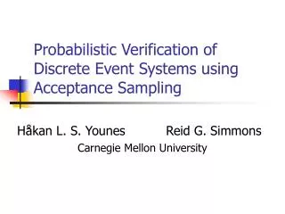
Acceptance Sampling and its Use in Probabilistic Verification Håkan L. S. Younes Carnegie Mellon University
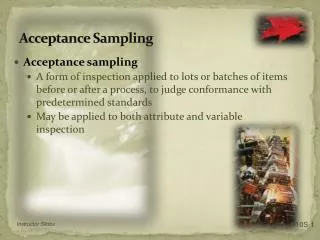
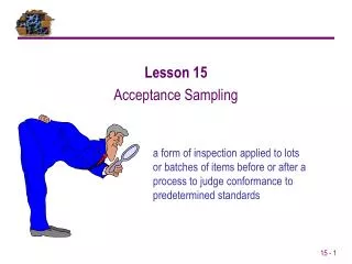
The Problem • Let be some property of a system holding with unknown probability p • We want to approximately verify the hypothesis p ≥ p’ using sampling • This problem comes up in PCTL/CSL model checking: Pr≥p’() • A sample is the truth value of over a sample execution path of the system
Quantifying “Approximately” • Probability of accepting the hypothesis p < p’ when in fact p ≥ p’ holds: ≤ • Probability of accepting the hypothesis p ≥ p’ when in fact p < p’ holds: ≤
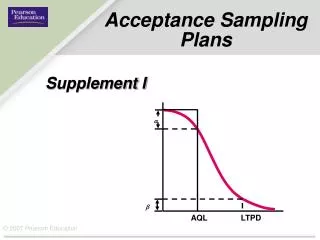
False negatives False positives Desired Performance of Test 1 – Unrealistic! Probability of acceptinghypothesis p ≥ p’ p’ Actual probability p of holding
Relaxing the Problem • Use two probability thresholds: p0 > p1 • (e.g. specify p’ and and set p0 = p’ + and p1 = p’ − ) • Probability of accepting the hypothesisp ≤ p1 when in fact p ≥ p0 holds: ≤ • Probability of accepting the hypothesisp ≥ p0 when in fact p ≤ p1 holds: ≤
False negatives Indifference region p1 p0 False positives Realistic Performance of Test 1 – Probability of acceptinghypothesis p ≥ p0 p’ Actual probability p of holding
Method 1:Fixed Number of Samples • Let n and c be two non-negative integers such that c < n • Generate n samples • Accept the hypothesis p ≤ p1 if at most c of the n samples satisfy • Accept the hypothesis p ≥ p0 if more than c of the n samples satisfy
Method 1:Choosing n and c • Each sample is a Bernoulli trial with outcome 0 ( is false) or 1 ( is true) • The sum of n iid Bernoulli variates has a binomial distribution
Method 1:Choosing n and c (cont.) • Find n and c simultaneously satisfying: • p’[p0,1], F(c, n, p’) ≤ • p’[0,p1], 1 - F(c, n, p’) ≤ • Non-linear system of inequalities, typically with multiple solutions! • Want solution with smallestn • Solve non-linear optimization problem using numerical methods p0) p1)
Method 1:Example • p0 = 0.5, p1 = 0.3, = 0.2, = 0.1: • Use n = 32 and c = 13 F(13, 32, p) 1 1 − Probability of acceptinghypothesis p ≥ p0 p1 p0 1 Actual probability p of holding
Idea for Improvement • We can sometimes stop before generating all n samples • If after m samples more than c samples satisfy , then accept p ≥ p0 • If after m samples only k samples satisfy for k + (n – m) ≤ c, then accept p ≤ p1 • Example of a sequential test • Can we explore this idea further?
True, false,or anothersample? Method 2:Sequential Acceptance Sampling • Decide after each sample whether to accept p ≥ p0 or p ≤ p1, or if another sample is needed
The Sequential Probability Ratio Test [Wald 45] • An efficient sequential test: • After m samples, compute the quantity • Accept p ≥ p0 if ≤ /(1 – ) • Accept p ≤ p1 if ≥ (1 – )/ • Otherwise, generate another sample
Accept Number of samplessatisfying Continue sampling Reject Number of generated samples Method 2:Graphical Representation • We can find an acceptance line and a rejection line give p0, p1, , and : Ap0,p1,,(m) Rp0,p1,,(m)
Accept Number of samplessatisfying Continue sampling Reject Number of generated samples Method 2:Graphical Representation • Reject hypothesis p ≥ p0 (accept p ≤ p1)
Accept Number of samplessatisfying Continue sampling Reject Number of generated samples Method 2:Graphical Representation • Accept hypothesis p ≥ p0
Method 2:Example • p0 = 0.5, p1 = 0.3, = 0.2, = 0.1: Number of samplessatisfying Number of generated samples
Method 2:Number of Samples • No upper bound, but terminates with probability one (“almost surely”) • On average requires many fewer samples than a test with fixed number of samples
Method 2:Number of Samples (cont.) • p0 = 0.5, p1 = 0.3, = 0.2, = 0.1: Method 1 Method 1 withearly termination Average number of samples Method 2 p1 p0 1 Actual probability p of holding
Acceptance Sampling with Partially Observable Samples • What if we cannot observe the sample values without error? • Pr≥0.5(Pr≥0.7(◊≤9 recharging) U≤6 have tea)
True, false,or anothersample? Acceptance Sampling with Partially Observable Samples • What if we cannot observe the sample values without error?
Modeling Observation Error • Assume prob. ≤ ’ of observing that does not satisfy a sample when it does • Assume prob. ≤ ’ of observing that satisfies a sample when it does not
Accounting forObservation Error • Use narrower indifference region: • p0’ = p0(1 – ’) • p1’ = 1 – (1 – p1)(1 – ’) • Works the same for both methods!
Observation Error: Example • p0 = 0.5, p1 = 0.3, = 0.2, = 0.1 • ’ = 0.1, ’ = 0.1 Average number of samples Number of samplessatisfying p1’ p0’ 1 Number of generated samples Actual probability p of holding
Application to CSL Model Checking [Younes & Simmons 02] • Use acceptance sampling to verify probabilistic statements in CSL • Can handle CSL without steady-state and unbounded until • Nested probabilistic operators • Negation and conjunction of probabilistic statements
Benefits of Sampling • Low memory requirements • Model independent • Easy to parallelize • Provides “counter examples” • Has “anytime” properties
… Polling stations Server CSL Model Checking Example: Symmetric Polling System • Single server, n polling stations • State space of size O(n·2n) • Property of interest: • When full and serving station 1, probability is at least 0.5 that station 1 is polled within t time units
105 104 103 102 101 100 10−1 10−2 102 104 106 108 1010 1012 1014 Symmetric Polling System (results) [Younes et al. ??] Pr≥0.5(true U≤t poll1) ==10−2 =10−2 Verification time (seconds) Size of state space
10 100 1000 Symmetric Polling System (results) [Younes et al. ??] Pr≥0.5(true U≤t poll1) 106 105 ==10−2 =10−2 104 Verification time (seconds) 103 102 101 100 t
Symmetric Polling System (results) [Younes et al. ??] Pr≥0.5(true U≤t poll1) 102 n=10 t=50 101 Verification time (seconds) ==10−10 ==10−8 ==10−6 100 ==10−4 ==10−2 0.001 0.01
Notes Regarding Comparison • Single state vs. all states • Hypothesis testing vs.probability calculation/estimation • Bounds on error probability vs. convergence criterion
Relevance to Planning [Younes et al. 03] • Planning for CSL goals in continuous-time stochastic domains • Verification guided policy search: • Start with initial policy • Verify if policy satisfies goal in initial state • Good: return policy as solution • Bad: use sample paths to guide policy improvement and iterate
Summary • Acceptance sampling can be used to verify probabilistic properties of systems • Have shown method with fixed number of samples and sequential method • Sequential method better on average and adapts to the difficulty of a problem