Capital Structure and Taxes

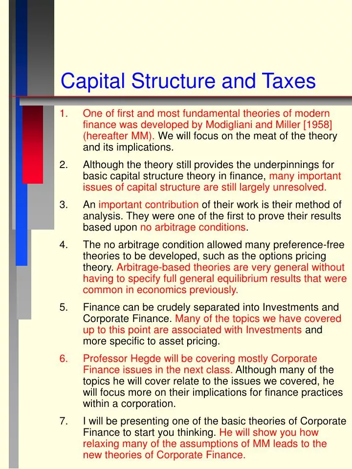
1. Capital Structure and Taxes • One of first and most fundamental theories of modern finance was developed by Modigliani and Miller [1958] (hereafter MM). We will focus on the meat of the theory and its implications. • Although the theory still provides the underpinnings for basic capital structure theory in finance, many important issues of capital structure are still largely unresolved. • An important contribution of their work is their method of analysis. They were one of the first to prove their results based upon no arbitrage conditions. • The no arbitrage condition allowed many preference-free theories to be developed, such as the options pricing theory. Arbitrage-based theories are very general without having to specify full general equilibrium results that were common in economics previously. • Finance can be crudely separated into Investments and Corporate Finance. Many of the topics we have covered up to this point are associated with Investments and more specific to asset pricing. • Professor Hegde will be covering mostly Corporate Finance issues in the next class. Although many of the topics he will cover relate to the issues we covered, he will focus more on their implications for finance practices within a corporation. • I will be presenting one of the basic theories of Corporate Finance to start you thinking. He will show you how relaxing many of the assumptions of MM leads to the new theories of Corporate Finance.

2. Simple Illustration of MM Theory • Before we look at the theory in mathematical form, the basis of the theory can be illustrated simply with the figure below. • 2. REMEMBER: The value of the firm is the discounted present value of it’s after-tax cash flows going to bondholders and stockholders. • 3. Two basic cases. • A. Without Income Taxes - income goes to • 1. stockholders • 2. bondholders • B. With Income Taxes - income goes to • 1. stockholders • 2. bondholders • 3. government.

3. In the second case, because interest paid on debt is tax deductible we can reduce the amount going to the government (and increase the amount going to bondholders and stockholders) by increasing the amount of debt in the capital structure. This should increase the value of the bondholders and stockholders claims.

4. 4. The initial paper by MM simply showed that the total value of the firm is the size of the pie. Changing the capital structure may change the size of the slice that goes to any group of claimants to the pie, but the size of the pie remains fixed given some simplifying assumptions. When there are no taxes and transactions costs, there is no way for a company to increase the value of a share or a bond by changing the capital structure. If there were, then an arbitrage would be possible. 5. MM won a Nobel prize for this work. One can argue that Coase (1960) won a Nobel prize for the same idea, but from a different perspective. He showed that in the absence of contracting costs and wealth effects, the assignment of property rights leaves the use of real resources unaffected. In other words, under the usual simplifying assumptions, assets will be allocated to their profit-maximizing use no matter who owns them. This shows how a clear understanding of the relatively few principals of economics (finance) can help you to understand many economic or financial problems.

5. Modigliani and Miller’s Initial Assumptions • Capital markets are frictionless – no transactions costs. • Everyone can borrow and lend at the riskless rate. • No bankruptcy costs. • Firms issue only riskless debt or risky equity. • All firms have the same risk. • Only corporate taxes may exist. • All cash flows are perpetuities. • Corporate insiders and outsiders have the same information. • Managers maximize shareholder wealth. • 1. With all cash flows perpetuities, the all-equity firm’s value is • Vu = E(FCF)/ • Where Vu = present value of the unlevered firm • E(FCF) = expected value of the firm’s free cash flow in each period forever into the future. •  = required return for an all equity firm given its risk.

6. 2. The definition of FCF FCF = (REV – VC – FCC – dep)(1 – tc) + dep – I Where REV = revenue, VC = variable costs, FCC = fixed cash costs such as administration costs, dep = depreciation and I = investment. Since we assume no growth, then dep = I so FCF = (REV – VC – FCC – dep)(1 – tc) = (NOI )(1 – tc) Under these assumptions, FCF ends up to be the same as net operating income after tax, which is also the cash flow the firm would have available if it had no debt. Therefore, firm value is Vu = E(NOI)(1 – tc)/ 3. Maintain the same assumptions but assume that the firm has debt = D on which it pays interest of kdD (kd is the coupon rate and D is the face value). The FCF is now split between interest payments to bondholders and net income (NI) to the equityholders. The only change to FCF is that interest payments provide a tax shield so that the total FCF increases by kdDtc,which is the reduction in taxes paid to the government simply because we have added bondholders. FCF = (NOI )(1 – tc) + kdDtc

7. 4. Assuming that the tax shield is a risk free cash flow, we can discount the tax shield using the before-tax risk free rate of kb, so that the value of the levered firm VL is, VL = E(NOI)(1 – tc)/ + kdDtc/kb Since the debt is a perpetual bond, its market value is B = kdD/kb so that VL = E(NOI)(1 – tc)/ + Btc It is clear that if there is no corporate tax (tc = 0), then the value of the firm will be unaffected by changes in the capital structure. This can be seen easily in, VL = Vu + Btc Furthermore, to maximize the levered firm value, the firm should increase the amount of debt as much as possible. Btc is the present value of the tax shield, sometimes called the “gain from leverage”.

8. MM’s Original Arbitrage Argument • Assume there are no taxes, then MM proved that there is no optimal capital structure. That is, firm value and equity value are unaffected by leverage. • To see this, assume that a levered firm and an unlevered firm are identical (same NOI) except that the levered firm has debt. Consider three portfolios. • Buy the fraction  of the equity Eu of the unlevered firm. • Buy the fraction  of the equity EL of the levered firm. Buy the fraction  of the debt D of the levered firm. • Buy the fraction  of the equity Eu of the unlevered firm. Borrow the amount D at the risk-free rate. • PortfolioActionInvestmentPayoff • __ ________________ • A Buy Unlevered Equity Eu NOI • B Buy Levered Equity EL(NOI – kdD) Buy Debt D (kdD) • Totals EL + D NOI • C Buy Unlevered Equity Eu NOI Borrow at risk free rate -D -(kdD) • Totals Eu - D NOI -(kdD)

9. 3. Compare portfolios A and B. Since Vu = Eu and VL = EL + D we see that each portfolio claims the fraction  in their respective firms. They receive the same payoff, NOI. By arbitrage, if the payoffs of the two portfolios is the same then the investment should also be the same, therefore, Vu = Eu = VL = EL + D 4. A second way to prove this is with portfolio C. This is called “homemade leverage” where the investor can produce his own leverage. This means that if anyone can do it, it can’t produce much value. Compare C’s total payoff to that of the levered equity in portfolio B. They are the same payoffs so the investments must be the same. If investment in portfolio C was less than the cost of the levered equity, investors would buy the unlevered equity and borrow until it forced the stock price up and the two investments were equal. Therefore, we must have EL = Eu - D So rearranging equating to firm values gives EL + D = VL = Eu = Vu

10. Weighted Cost of Capital • To get the cost of capital for a levered firms, we can consider the change in company value due to the change in investment as follows: • VL = E(NOI)(1 – tc) + B tc = 1 II  I • We set this equal to one because at the margin, an additional $1 in investment increases the company’s value by $1 since for the marginal investment NPV = 0. That is, VL = I . From this we get • (1 – tc)E(NOI) = ( 1 - tc[B/I]) = ( 1 - tc[B/VL]) I • The first term is the after-tax change in net operating cash flows due to the investment – the after-tax return on the project. The next two terms are the opportunity cost of capital for the project. Therefore, the weighted average cost of capital (WACC) is • WACC = ( 1 – tc[B/VL]) • We can see that if there is no tax, then the cost of capital is fixed no matter what the capital structure. If there is tax, then the cost of capital decreases as we add more debt to the capital structure. • This equation defines the cost of capital relative to the all-equity cost of . With taxes, the debt tax shield reduces the average cost, and a higher tax rate means a lower capital cost, as the government subsidizes investment.

11. The Traditional Definition of WACC • To get the traditional WACC from the definition above, we assume, like MM, that [B/I] = [B/VL] = [B/ VL]. This just means that the marginal use of debt to finance new investments equals the average use of debt in the capital structure. • We have already assumed that debt pays the risk-free return and since VL = EL + B, then • cost of debt = (1 – tc)kb[B/(EL + B)] • with WACC = ( 1 – tc[B/VL]) =  -  tc[B/(EL + B)] • Add and subtract the cost of debt from RHS to get • WACC = (1 – tc)kb[B/(EL + B)] +  -  tc[B/(EL + B)] - (1 – tc)kb[B/(EL + B)] • Now combine the last 3 terms and note that [B/(EL + B)] = [B/EL] [EL/(EL + B)]

12. Now we have the WACC in the traditional form where the weights are the proportions of debt and equity in the capital structure. This means that the required rate of return for equity for a leveraged firm is KE =  + (1 – tc)( - kb)[B/EL] Here we see that the required return decreases with an increase in the tax rate and increases with an increase in debt relative to equity. Now we can combine the cost of debt and equity to get:

13. The graphs above illustrate how the cost of equity and the WACC changes with leverage. • Graph (a) shows that with no taxes the WACC stays constant because the cost of equity rises to exactly offset the lower cost of debt as more debt is added to the capital structure. • Graph (b) shows that with taxes, the cost of equity rises but not as steeply as when there are no taxes. Therefore, as cheap debt is added to the capital structure, the WACC falls.

14. Traditional Theory of Cost of Capital • The traditional theory of WACC had little rigorous theory to support it. It was assumed that as one added cheap debt to the capital structure, WACC would fall. • But at some point, it was assumed that the probability of bankruptcy would rise so high that the WACC would increaseas lenders and stockholders required higher returns.

15. Two Capital Structure Theories of Leverage a. Traditional - Share Price will Increase with Leverage up to a Point (Too Much Risk) b. Net Operating Income Theory (MM) - Any Increase in Leverage and EPS will be Offset by Increased Risk (Assuming No Taxes) Leaving the Share Price Unchanged. Illustration using the constant growth model. P = D1/ (kE - g) Increasing leverage may increase D1 and g but will increase beta (risk) so that kE will increase. Theoretically, P stays the same because the positive effect of the increase in D1 and g is just offset by the negative effect of the kE increase.

16. MM With Personal Taxes as Well as Corporate Taxes • Miller (1977) shows how personal taxes on stock income of ts and on bond income tb can change the effects of leverage on the WACC. The value of the unlevered firm will be • Vu = E(NOI)(1 – tc)(1 – ts)/ • Here, the numerator is now the shareholder income after corporate and personal income taxes. For the levered firm we have • VL = E(NOI)(1 – tc)(1 – ts)/ + kdD[(1 – tb) - (1 – tc)(1 – ts)]/kb • Since B = kdD(1 – tb)/kb then • VL = Vu + [1 - (1 – tc)(1 – ts)/(1 – tb)]B • Now the gain from leverage is likely to be smaller because we typically have a smaller tax rate on stock income than bond income, i.e., ts < tb. If ts = tb then we have the same formula as without personal taxes. • If (1 – tc)(1 – ts) = (1 – tb), then there is no gain from debt, the positive effect of corporate tax deductibility is offset by the large personal tax on bond income. • When this occurs, the tax rate on bonds is so large relative to stocks that bondholders demand a very large before-tax rate of return. This forces interest payments up enough so that even after corporations deduct the interest, it is cheaper to use equity than debt.

17. Example: SI Inc. is an all-equity firm that generates EBIT of $3 million per year. Its cost of equity capital is 16 percent, its marginal corporate tax rate is 35 percent, and it has 1 million shares outstanding. a What is SI’s market value? b. If SI issues $4 million of debt and uses it to buy back some shares, what will be its new market value and new equity value? c. Show that the change in per-share value goes up even though total equity decreases. a. Vu = $3,000,000(1 - .35) / .16 = $12,187,500 b. VL = $12,187,500 + (.35)($4,000,000)=$13,587,500 equity = $13,587,500 - $4,000,000 = $9,587,500 c. Before buyback, share price= $12,187,500/1,000,000 = 12.187 After buyback of $4,000,000/12.187 = 328,218 shares we get a new price of P =$9,587,500/(1,000,000 - 328,218) = 14.27

18. Synthesis of MM and CAPM • MM assumed that all firms had the same risk. One way to relax this assumption is to combine MM and the CAPM. The CAPM defines required returns for assets with different risks. Both MM and the CAPM give us a definition for the cost of equity capital. We can merge these definitions and gain some insights. • For a leveraged firm we have • KE =  + (1 – tc)( - kb)[B/EL] = Rf + [E(Rm) – Rf]L • Now substitute for kb = Rf and  = Rf + [E(Rm) – Rf]u and rearrange to get • L = [1 + (1 – tc)(B/EL)] u • The value of this expression is that if we know the levered beta we can get the unlevered beta or vise versa. We can also see that the levered beta decreases with the tax rate and increases with the debt level. • NOTE: It is usually assumed that there is an optimal capital structure so that (B/EL) is the same for all projects. Then, the decision to invest in a project is only dependent on its risk and potential cash flows. But if a project is special because it can be financed with greater debt capacity than alternative projects, then the investment decision will affect the capital structure, which in turn, affects the risk of the project and its required return.

19. MM and the follow-on papers show that many financial practices, and capital structure manipulation in particular, are unlikely to increase firm value. • In order to show that a practice has value, one must show either that it increases net cash flows to shareholders or decreases firm risk or both and that investors cannot perform the manipulation on their own. • In the 1960’s, many conglomerate mergers were conducted because it was believed that the net risk of the combined firms would fall. By the 1980’s, many mergers proved to be bad for shareholders. First, investors could always combine firm shares on their own to achieve diversification. Second, the combined firms often were inefficient because management could not run two business well at the same time. Recently, researchers are reconsidering when mergers are valuable and when they are not. • The use of derivatives to manage a firm’s risk is another case in point. Should corporate managers be using futures, options and swaps to hedge risk or add risk? The argument against says that corporate managers should concentrate on running their businesses – they will reduce value by trying to use derivatives they are not expert in. The argument in favor says that corporate managers should know which risks they are expert in and which risks it is best to let others bear. The firm should only keep risks for which it thinks it can earn an acceptable return.

20. Possible Reasons for Different Capital Structures • Bankruptcy costs may be substantial, including legal costs, lost real options, lost customer relations, and bondholder-stockholder conflict costs. • Transactions costs may be substantial, including large homemade leverage costs for shareholders, margin expenses and shortsale restrictions. • Investors may face a different tax rate than corporations and different levels of progression. • Imperfect information may make it difficult for shareholders to undo company leverage or properly monitor firm managers. Capital structure may be used as an incentive tool for managers to work hard – more debt – more pressure on management to produce good returns or else face bankruptcy and being fired. Implies – add a slice to the earlier pie chart where the slice goes to management or covers management inefficiencies – then argue that more debt reduces this slice, giving more to bondholders and stockholder. But it seems that this could be handled with incentive compensation and monitoring instead of taking on more debt and, therefore, bankruptcy risk.

21. Steven Ross, The Determinants of Financial Structure: The Incentive Signal Approach, (Bell Journal of Economics, 1977) Separating Equilibrium: A signaling mechanism arises naturally in the market to signal information to market participants which allows them to “separate” or determine which firms have good future prospects and which don’t. Ross suggests that MM’s assumption that all market participants know what future firm cash flows will be is wrong. Asymmetric information - managers know more than investors. Assume managers can’t trade their own stock. Managers can use the firm’s capital structure to signal. Manager compensation (M) is, Where 0 and 1 are positive constants r is the one period interest rate V0=V1/(1+r) and V1 are the current and future firm values D is the face value of firm debt C is a penalty paid if bankruptcy occurs (V1 < D)

22. Assumptions 1. There are two types of firms, a successful type A and an unsuccessful type B, and the value of type A greater than the value of type B. Va > Vb 2. D* is the maximum amount of debt that an unsuccessful firm can carry without going bankrupt. 3. D > (<) D* means management signals it is type A (B). For a signaling equilibrium, management compensation must be such that managers of type A firms and type B firms make more if they truthfully signal their firm’s type. For type A and then type B, the manager compensation is

23. Results of model – similar to many other signaling results, e.g. dividends etc. 1. Clearly, managers of firms of type A will tell the truth by choosing D > D* because they earn more compensation if they do because Vb < Va. 2. Managers of type B firms don’t necessarily have the same incentives. Compensation must be set such that they earn more by correctly choosing D < D* to signal that they are type B. This is true when Or This condition says that the management compensation gain from lying must be less than the management compensation loss. The LHS is the management share of gain from initially fooling the market that it is a type A when it is really a type B. The RHS is the penalty due to bankruptcy.

24. Unsuccessful firms don’t have enough cash to avoid bankruptcy if D > D* and lying managers will earn less, therefore, a signaling equilibrium accurately separates firms into high-priced (P = Va ) and low-priced (P = Vb). Without this signaling, all of the firms will trade at the same price because investors cannot distinguish one from another. If half of the firms are type A and half type B, then the market price for all firms will be P = .5 Va + .5 Vb. To get the price of equity, one needs to subtract the value of the debt in each case.