Download
1 / 41
410 likes | 443 Views
Delve into the fascinating realm of oceanography with a focus on properties of seawater, T-S distribution, fluid dynamics, large-scale gyres, mixing, and more. Join us for an in-depth study of Earth's oceans. Learn through lectures, readings, assignments, exams, and projects to enhance your understanding of this dynamic field.

E N D
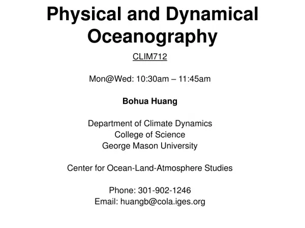
Physical and Dynamical Oceanography CLIM712 Wednesday: 10:30am – 1:15pm Bohua Huang Department of Atmospheric, Oceanic, and Earth Sciences College of Science George Mason University Center for Ocean-Land-Atmosphere Studies Phone: 301-902-1246 Email: huangb@cola.iges.org bhuang@gmu.edu
References Text books: • Pond, S., and G.L. Pickard, 1983: Introductory Dynamical Oceanography. 2nd edition, 329pp, Butterworth-Heinemann. • Pickard, G.L., and W.J. Emery, 1993: Descriptive Physical Oceanography, 5th enlarged edition, 320pp, Pergamon Press. Other titles of interest: • Mellor, G.L., 1996: Introduction to Physical Oceanography, 260pp, AIP Press. • Knauss, J.A., 1997: Introduction to Physical Oceanography, 309pp, 2nd edition, Prentice-Hall. • McWilliams, J.C., 2006: Fundamentals of Geophysical Fluid Dynamics, 249pp, Cambridge, More readings: • Tomczak, M., and J.S. Godfrey, 1994: Regional Oceanography: An Introduction, 422pp, Pergamon Press. • Abarbanel, H.D.I., and W.R. Young, Eds., 1987: General Circulation of the Ocean, 291pp. Springer-Verlag. • Warren, B.A., and C. Wunsch, Eds., 1981: Evolution of Physical Oceanography, 623pp, The MIT Press. • Pedlosky, J., 1996: Ocean Circulation Theory, 453pp, Springer. • Siedler,G., J. Church, and J. Gould, Eds., 2001: Ocean Circulation and Climate, 715 pp., Academic Press.
Useful Websites Physical Oceanography Courses • R. H. Stewart:Introduction to Physical Oceanography (http://oceanworld.tamu.edu/resources/ocng_textbook/contents.html) • M. Tomczak: Introduction to Physical Oceanography(http://gaea.es.flinders.edu.au/~mattom/IntroOc/newstart.html) • B. A. Warren & C. Wunsch (Ed.,): Evolution of Physical Oceanography (http://ocw.mit.edu/ans7870/resources/Wunsch/wunschtext.htm) • M. Tomczak, & J. S. Godfrey: Regional Oceanography: an Introduction (http://gaea.es.flinders.edu.au/~mattom/regoc/index.html) • F. Webster: Introduction to Physical Oceanography (http://www.cms.udel.edu/mast602)
Requirement • Regular classes • Homework: 5-6 assignments • NOAA monthly ocean briefing • Mid-term exam (close book) • Final exam (open book) • Project (term paper) Slides of the lectures will be on: ftp://grads.iges.org/pub/huangb/Fall09 before each class
Major Topics • Properties of seawater • T-S forcing and conservation laws • Global T-S distribution • Fluid dynamics on rotating sphere • Description of large-scale gyres • Barotropic dynamics of large-scale gyres • Mixing, turbulence, surface layer • Large-scale overturning and thermohaline circulation • Surface gravity waves (nonrotating and rotating) • Internal gravity waves • Rossby waves, instability and mesoscale eddies • Tides • Coastal processes: currents, fronts, estuaries • El Nino
Course Outline [Numbers in brackets give chapters to read in Descriptive Physical Oceanography, 5th Ed.(Des), and Introductory Dynamical Oceanography, 2nd Ed.(Dyn). Lectures do not cover the entirety of all chapters assigned; students will only be responsible for material covered in lectures. For some topics, additional reading materials will be supplied with class notes] • Properties of seawater [Des 2, 3, 6] • composition • equation of state • measurement: T, S, pressure • Global T-S distribution [Des 4 ] • surface profiles • vertical profiles • static stability • annual cycle and interannual variability • T-S Forcing and conservation laws [Des 5] • heat flux components • heat flux distribution • evaporation, precipitation, runoff • box models • Fluid dynamics on rotating sphere [Dyn 6, 8, 9.1-9.4] • Coriolis force • equations of motion • geostrophy • Ekman layers • Description of large-scale gyres [Des 7] • wind patterns and gyres • western and eastern boundary currents • polar currents • equatorial currents • Barotropic dynamics of large-scale gyres [Dyn 9.5-9.14] • vorticity dynamics • gyres and western boundary currents • Sverdrup, Stommel, and Munk
Mixing, turbulence, surface layer [supplied reading] - descriptive Kelvin-Helmholtz instability - surface mixed layer dynamics - sources of subsurface mixing • Large-scale overturning [supplied reading] - thermohaline structure and meridional overturning - advective-diffusive balance and overturning - Stommel-Arons patterns - subduction and shallow cells • Surface gravity waves (nonrotating and rotating) [Dyn 12.1-12.8, 12.10.1-12.10.3] - short and long nonrotating SGWs - Poincare and Kelvin waves • Tides [Dyn 13.1-13.7] - tidal forcing - equilibrium theory - forced response • Internal gravity waves [Dyn 12.9] - two-layer fluid - rotational effects - continuous fluid • Rossby waves, instability and mesoscale eddies [supplied reading] - Rossby wave dynamics - observations of eddies • Coastal processes: currents, fronts, estuaries [Des 8] • El Nino [supplied reading] - air-sea feedbacks - equatorial waveguide - ENSO description
Introduction Why is ocean important for climate? What is Physical Oceanography? How do we do it? A brief history
Ocean plays important roles in maintaining the earth climate •Ocean has large heat storage -- Roughly, 3 meters of sea water has about the same heat capacity as the whole atmospheric column above it -- Ocean heat storage modulates diurnal and seasonal cycles and climate variations -- Maritime climate is generally milder than continental climate
• Ocean transfers heat and freshwater over a wide range of time and space scales -- The earth system is not in radiative balance -- The tropics gaining and the polar regions losing heat -- Meridional oceanic heat transport is comparable to that of the atmosphere
Fluctuations within the ocean affect the climate significantly. Sea surface temperature (SST) changes from year-to-year significantly. The SST anomalies can persist for a long time.
The SST anomalies have serious consequences to the weather and climate
Air-sea interaction is an important source for global climate variability (e.g., ENSO) Ocean provides the “memory” of the low frequency fluctuations
ocean plays a significant role in the global change. The figure depicts atmospheric CO2 concentrations from 1958 to the present as measured at Mauna Loa, Hawaii. These data, obtained by Keeling and Whorf (1998), represent the longest continuous record of directly measured CO2 concentrations. As the graph of these data indicates, there has been a substantial and sustained rise in the air's CO2 content over the past four decades, from about 315 ppm to over 360 ppm. The greenhouse effect tends to increase atmospheric temperature. Ocean is a major part of global carbon cycle and our knowledge of oceanography may be important for estimating the trend of global warming.
Figure 5.1. Time series of global annual ocean heat content (1022 J) for the 0 to 700 m layer. The black curve is updated from Levitus et al. (2005a), with the shading representing the 90% confidence interval. The red and green curves are updates of the analyses by Ishii et al. (2006) and Willis et al. (2004, over 0 to 750 m) respectively, with the error bars denoting the 90% confidence interval. The black and red curves denote the deviation from the 1961 to 1990 average and the shorter green curve denotes the deviation from the average of the black curve for the period 1993 to 2003 (IPCC Report).
It is possible that much of the rise in sea level has been related to the concurrent rise in global temperature over the last 100 years. On this time scale, the warming and the consequent thermal expansion of the oceans may account for about 2-7 cm of the observed sea level rise, while the observed retreat of glaciers and ice caps may account for about 2-5 cm.
Figure 5.13. Annual averages of the global mean sea level (mm). The red curve shows reconstructed sea level fields since 1870; the blue curve shows coastal tide gauge measurements since 1950 and the black curve is based on satellite altimetry). The red and blue curves are deviations from their averages for 1961 to 1990, and the black curve is the deviation from the average of the red curve for the period 1993 to 2001. Error bars show 90% confidence intervals (IPCC Report). Figure 5.14. Variations in global mean sea level (difference to the mean 1993 to mid-2001) computed from satellite altimetry from January 1993 to October 2005, averaged over 65S to 65N. Dots are 10-day estimates (from the TOPEX/Poseidon satellite in red and from the Jason satellite in green). The blue solid curve corresponds to 60-day smoothing (IPCC Report).
Global ocean circulation may be changed fundamentally by climate change And the oceanic circulation change will feedback seriously to the earth climate.
Figure 10.15. Evolution of the Atlantic meridional overturning circulation (MOC) at 30∞N in simulations with the suite of comprehensive coupled climate models (see Table 8.1 for model details) from 1850 to 2100 using 20th Century Climate in Coupled Models (20C3M) simulations for 1850 to 1999 and the SRES A1B emissions scenario for 1999 to 2100. Some of the models continue the integration to year 2200 with the forcing held constant at the values of year 2100. Observationally based estimates of late-20th century MOC are shown as vertical bars on the left. Three simulations show a steady or rapid slow down of the MOC that is unrelated to the forcing; a few others have late-20th century simulated values that are inconsistent with observational estimates. Of the model simulations consistent with the late-20th century observational estimates, no simulation shows an increase in the MOC during the 21st century; reductions range from indistinguishable within the simulated natural variability to over 50% relative to the 1960 to 1990 mean; and none of the models projects an abrupt transition to an off state of the MOC. Adapted from Schmittner et al. (2005) with additions (IPCC report).
Figure 10.16. Base state change in average tropical Pacific SSTs and change in El NiÒo variability simulated by AOGCMs (see Table 8.1 for model details). The base state change (horizontal axis) is denoted by the spatial anomaly pattern correlation coefficient between the linear trend of SST in the 1% yr-1 CO2 increase climate change experiment and the first Empirical Orthogonal Function (EOF) of SST in the control experiment over the area 10S to 10N, 120E to 80W (reproduced from Yamaguchi and Noda, 2006). Positive correlation values indicate that the mean climate change has an El Nino-like pattern, and negative values are La Nina-like. The change in El Nino variability (vertical axis) is denoted by the ratio of the standard deviation of the first EOF of sea level pressure (SLP) between the current climate and the last 50 years of the SRES A2 experiments (2051-2100), except for FGOALS-g1.0 and MIROC3.2(hires), for which the SRES A1B was used, and UKMO-HadGEM1 for which the 1% yr-1 CO2 increase climate change experiment was used, in the region 30S to 30N, 30E to 60W with a five-month running mean (reproduced from van Oldenborgh et al., 2005). Error bars indicate the 95% confidence interval. Note that tropical Pacific base state climate changes with either El NiÒo-like or La Nino-like patterns are not permanent El Nino or La Nina events, and all still have ENSO inter- annual variability superimposed on that new average climate state in a future warmer climate.
ocean circulation and marine biology -- T and S distribution affects phytoplankton -- Current affects the concentration and dispersion -- Mixing and upwelling are important to provide nutrients -- Phytoplankton changes the ocean color -- Phytoplankton represents the first link in the marine food web -- Phytoplankton has a major role in the global carbon cycle -- An indicator of circulation change -- Biological feedback to circulation?
Ocean Color and El Niño As indicated by the red (warm) region off the west coast of Peru (top image), El Niño was still going strong in February 1998. Phytoplankton were growing just to the north of the equator (bright blue green region in the image second from top). By February 1999 La Niña had replaced El Niño, and the equatorial Pacific had strong phytoplankton production (bottom pair of images). Images by Robert Simmon based on data from the Distributed Active Archive Centers at the JPL and GSFC
Knowledge of ocean circulation, especially coastal processes, is helpful for environmental sciences -- pollution -- oil drilling -- oil spills -- sewage outfalls -- industrial waste
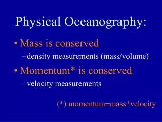
What is Physical Oceanography? 1). A description of the temperature, salinity, and density patterns in the ocean, including their variability. 2). The three dimensional water movement (the circulation: currents and vertical movements; also, waves and tides). 3). The transfer of mass, energy, and momentum between the ocean and the atmosphere. 4). The special properties of sea water (e.g., the propagation of sound and light energy). 5). The mechanisms of these properties and processes. Simply: • What temperature is the water? • What salinity is the water? • Where is the water going? • Why is that?
The approach of physical oceanography research • observations to get the basic phenomenon • applying laws of physics to explain the features we find (hypothesis/theory) • theory leads us to find new information to verify its predictions (more observation) • new observations test (verify, modify, or disprove) the theory (improved theory) • general circulation models blurs the boundary between traditional physical and dynamical branches
Figure 1.1 Data, numerical models, and theory are all necessary to understand the ocean. Eventually, an understanding of the ocean-atmosphere-land system will lead to predictions of future states of the system (From Stuart 2007).
Gulf Stream: An ExampleQuestions:Why does the Gulf Stream concentrate near the western boundary?What determines its width and speed?Why are there meanders and rings?Any climate significance?…….
A Brief History of Oceanographic Exploration Surface Oceanography- major approach prior to 1873 Systematic collection of phenomena observable from the deck of sailing ships (marine winds, currents, waves, temperature etc.) Examples: Halley’s charts of the trade-winds (1685); Hadley(1735) Franklin’s map of the Gulf Stream (1769) Maury's Physical Geography for the Sea (1847) Pillsbury's measurements of the Florida Current (1885)
Oceanographic Expeditions Wide range survey of surface and subsurface oceanic conditions Examples: Challenger Expedition (British, 1872-1876) Main interest in marine life below 600 m but also collected large amount of physical measurements in the Atlantic and Pacific Fram Expedition (Norway, 1895-1896) Leaded by Nansen, polar sea exploration Meteor Expedition (German, 1925-1927) Leaded first by Merz and later by Wüst, concentrated on overturning circulation. The ship travels 67,000 miles, made 14 sections across the Atlantic, 310 hydrographic stations, 33,000 depth sounding Other Acchivements The Scandinavian Scientists developed the “dynamical method” to derive geostropic currents from T-S observations Reversing thermometer gives more accurate subsurface temperature measurements
Upper panel: Track of the H.M.S. Challanger during the British Challanger Expedition 1872-1876. From Wüst (1964). Right panel: Track of the R/V Meteor during the German Meteor Expedition. From Wüst (1964).
International Programs: 1957-1978 • Multi-national surveys of oceans and studies of oceanic processes. Example: International Geophysical Year cruises • Multiship studies of oceanic processes: e.g., MODE, POLYMODE experiments •New Technologies improve observations significantly Bruce Hamon and Neil Brown develop the CTD for measuring conductivity and temperature as a function of depth in the ocean (1955). Sippican Corporation (Tim Francis, William Van Allen Clark, Graham Campbell, and Sam Francis) invents the Expendable Bathy Thermograph (XBT), now perhaps the most widely used oceanographic instrument (1963).
The sections in the International Geophysical Year Atlantic Program 1957-1959. From Wüst (1964).
Satellite Remote Sensing (since 1978) Examples Seasat (1978) NOAA 6-17 (1979-2002) NIMBUS-7 (1978-1994) Geosat (1985-1990) Topex/Poseidon (1992-) ERS 1 & 2(1991-00, 1995) Global surveys of oceanic processes from space Topex/Poseidon tracks in the Pacific Ocean during a 10-day repeat of the orbit. From Topex/Poseidon Project.
Earth System Study Global studies of the interaction of biological, chemical, and physical processes in the ocean, the atmosphere and the land using in situ and space data as well as coupled models. Oceanic examples Tropical Ocean-Global Atmosphere (TOGA) Program (1985-1995) World Ocean Circulation Experiment (WOCE, 1991-1996) Joint Global Ocean Flux Study (JGOFS)
World Ocean Circulation Experiment: Tracks of research ships making a one-time global survey of the oceans of the world
Some Theoretical Milestones • 1775 Laplace's published his theory of tides. • 1800 Rumford proposed a meridional circulation of the ocean with water sinking near the poles and rising near the Equator. • 1905 Ekman published his paper on wind-driven oceanic boundary layer. • 1910-1913 Vilhelm Bjerknes published Dynamic Meteorology and Hydrography which laid the foundation of geophysical fluid dynamics. • 1942 Publication of The Oceans by Sverdrup, Johnson, and Fleming, the first comprehensive survey of oceanographic knowledge. • 1947-1950 Sverdrup, Stommel, and Munk publish their theories of the wind-driven circulation of the ocean. Together the three papers lay the foundation for our understanding of the ocean's circulation. • 1958 Stommel publishes his theory for the deep circulation of the ocean. • 1969 Kirk Bryan and Michael Cox develop the first numerical model of the oceanic circulation. • ……