Image Compression
This detailed overview covers image compression methods like lossless and lossy, coding redundancy, quantization, symbol encoding, and compression algorithms such as Huffman coding and Run-Length Encoding. Learn about techniques, measurements of distortion, and strategies for effective image data reduction.

Image Compression
E N D
Presentation Transcript
Image Compression Attempts to exploit the presence of redundant information in images - coding redundancy - spatial redundancy - spectral redundancy - temporal redundancy - psychovisual redundany
Image Compression Goal: identify a representation for the data in which the redundancy is decreased - find a more compact representation - a representation in which most of the information is contained within relatively few values
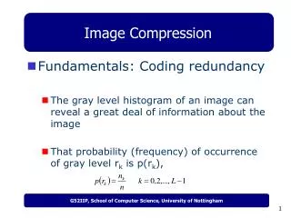
Coding Redundancy G - 1 Avg code length = len (codek) p (codek) (for a pixel value) k = 0 length of codek probability of codek For an uncompressed n-bit image code length = n, independent of probability
Coding Redundancy G - 1 Avg code length = len (codek) p (codek) (for a pixel value) k = 0 Variable length codes reduce average code length by assigning shorter codes to more probable pixel values
Image Compression LOSSLESS - bit-preserving or reversible compression. The reconstructed image is numerically identical to the original LOSSY - irreversible compression. Information has been lost in the compression process. The reconstructed image is numerically different than the original.
LOSSY COMPRESSION: Information which is lost during the compression process produces distortion or differences between the original and the reconstructed image
ORIGINAL IMAGE DECOMPOSITION OR TRANSFORMATION QUANTIZATION SYMBOL ENCODING COMPRESSED IMAGE
ORIGINAL IMAGE DECOMPOSITION OR TRANSFORMATION QUANTIZATION SYMBOL ENCODING COMPRESSED IMAGE Information is often lost in the quantization stage of compression
N M RMSE = ( f(x,y) - g(x,y) ) x=1 y=1 reconstructed image original image 255 RMSE PSNR = 20 log 10 1 MN Numeric Measures of Distortion 2 A high PSNR indicates a good reconstruction
original image half intensity image PSNR = 11.5dB
original image subsampled, enlarged image PSNR = 19.5dB A higher PSNR is not always indicative of a higher quality image
Coding Algorithms • - Run-Length Encoding (RLE) • - Huffman Coding • Bit Plane Coding • - Gray Code
Huffman Coding Variable length coding: construct variable length codes that assign the shortest possible code words to the most probable gray levels When coding symbols individually, Huffman coding yields the smallest number of code symbols per source symbol.
Huffman Coding Step 1: Create a series of source reductions by ordering the probabilities of the symbols, and combining the lowest probability symbols into a single symbol that replaces them at the next source reduction. Step 2: Code each reduced source starting with the smallest source and working back to the original source
1 1 1.0 0.2 1 0 0 0.3 1 1 0.1 0 0.6 0 0 A1=0111 A2=1 A3=0101 Collecting the binary digits from right to left: A4=0110 A5=0100 A6=00 Huffman Coding Symbol Probability A1 0.1 A2 0.4 A3 0.06 A4 0.1 A5 0.04 A6 0.3
Run-length Encoding - supported by many bitmap file formats (TIFF, BMP, PCX) - easy to implement - quick to execute - compression efficiency depends on the content of image data being encoded.
Run-length Encoding RLE works by reducing the physical size of a repeating string of characters. This repeating string, called a run, is typically encoded into two bytes: run count - # of characters in the run run value -value of the character in the run
Run-length Encoding With 8-bit image data: - run may contain 1 to 256 characters - run count usually contains the number of characters minus one (a value in the range of 0 to 255). - value of the character in the run, which is in the range of 0 to 255
Run-length Coding for 1-Bit (binary) Image Data Standard compression approach for FAX transmission (along with 2-D extensions) Code the length of each contiguous group of 1’s or 0’s encountered in the left to right scan of a row. Often a convention is used to determine the value of the run. For example, all rows begin with a white run, sometimes of length zero.
Run-length Encoding Additional compression can be achieved by variable length coding the run lengths themselves. Black and white run lengths may be coded separately using variable length codes tailored to their own statistics.
Bit Plane Encoding we decompose an NxN k bit image into k, NxN bit planes (numbered 0 through k-1) simple approach: mask each plane by logically ANDing each pixel value with 2 , for i = 0,..,k-1 f 7(x,y) = f(x,y) AND 1000000 f 6(x,y) = f(x,y) AND 0100000 ... f 1(x,y) = f(x,y) AND 0000001 i
Bit Plane Encoding f 7(x,y) = f(x,y) AND 1000000 f(x,y)
Bit Plane Encoding f(x,y) AND 0100000 f(x,y) AND 1000000 f(x,y) AND 0001000 f(x,y) AND 0010000
Bit Plane Encoding - enables efficient use of binary compression techniques (Run Length Encoding) - facilitates progressive coding and transmission
Bit Plane Encoding problem: binary representations do not take advantage of coherency (existence of large uniform areas) example: pixel values 127 and 128 very similar in value very different in binary representation 01111111 and 10000000
Bit Plane Encoding problem: binary representations do not take advantage of coherency (existence of large uniform areas) solution: gray code. Gray code representations of values which differ by one, differ by exactly 1 bit
Bit Plane Encoding mapping from binary to gray code: 1) starting with MSB of binary code, all 0’s are left intact until a 1 is encountered 2) The 1 is left intact, but all following bits are complemented until a 0 is encountered 3) The 0 is complemented, but all following bits are left intact until a 1 is encountered 4) Goto step 2
Binary Code Gray Code Bit plane 7 Bit plane 6
Binary Code Gray Code Bit plane 5 Bit plane 4
Grey Level Quantization reduce a k bit representation to a p bit representation by keeping only the p highest bits of the pixel value fp(x,y) = fk(x,y) / 2 (k-p)
Grey Level Quantization 8 bit pixel value -> 4 bit pixel value f4(x,y) = f8(x,y) / 2 = f8(x,y) / 16 to uncompress: f4(x,y) * 16 or f4(x,y) * 16 + 8 (8-4)
Grey Level Quantization Quantized - 4 bit image (PSNR 28.65 dB) Original - 8 bit image
Grey Level Quantization Quantized - 4 bit image (PSNR = 28.75 dB) Original - 8 bit image
Grey Level Quantization reduce a k bit representation to a p bit representation by keeping only the p highest bits of the pixel value fp(x,y) = (fk(x,y) + randome) / 2 where the random value e is a random number whose average value is equal to the average error incurred in the quantization process. (k-p)
Grey Level Quantization Quantized - 4 bit image with random additive noise (PSNR = 27.49 dB) Original - 8 bit image
Grey Level Quantization Quantized - 4 bit image with random additive noise (PSNR = 27.49 dB) Quantized - 4 bit image (PSNR = 28.75 dB)
JBIG Compression Joint Bi-level Image Experts Group • Lossless compression of one-bit-per-pixel image data • Ability to encode individual bitplanes of multiple-bit pixels • Progressive or sequential encoding of image data
JBIG Compression - uses a two-dimensional template of patterns in a binary image In the above, a neighborhood of seven pixels is used as a predictor. Probability of a zero is initially 0.5, but is corrected adaptively as the mage is encoded.
JPEG Compression (Joint Photographic Experts Group) - not a single algorithm, but a toolkit of image compression methods - lossy method of compression. - based on the Discrete Cosine Transform (DCT) - uses a quality setting or a Q factor. (Typically a range of 1 to 100: A factor of 1 produces the worst quality images; a factor of 100 produces the best quality images. )
JPEG Compression 1 - Transform the image into an optimal color space. 2 - Downsample chrominance components by averaging groups of pixels together. 3 - Apply a Discrete Cosine Transform (DCT) to blocks of pixels, thus removing redundant image data. 4 - Quantize each block of DCT coefficients using weighting functions optimized for the human eye. 5 - Encode the resulting coefficients (image data) using an adaptive Huffman coder.
JPEG Compression 1) image is divided into 8x8 blocks of pixels 2) a DCT is applied to each 8x8 block: - first term is the average - each successive term represents the strength of higher frequency components 3) the coefficients of each block are quantized (its value is represented with less accuracy) 4) quantized value is encoded (huffman or arithmetic coding)
JPEG Compression original 6:1 compression PSNR = 34.56 dB
JPEG Compression original 42:1 compression PSNR = 22.44 dB
Lempel-Ziv-Welch (LZW) Compression - used in several image file formats, such as GIF and TIFF - generally fast in both compressing and decompressing data - because LZW writes compressed data as bytes and not as words, LZW-encoded output can be identical on both big-endian and little- endian systems,
Lempel-Ziv-Welch (LZW) Compression - referred to as a substitutional or dictionary- based encoding algorithm. - The algorithm builds a data dictionary of data occurring in an uncompressed data stream (image). - each entry in the dictionary contains a pattern and a code phrase
Lempel-Ziv-Welch (LZW) Compression - Patterns of data (substrings) are identified in the image and are matched to entries in the dictionary. - If a data pattern is found in the dictionary, the corresponding code phrase is written to the output. - If the pattern is not found in the dictionary, a new code phrase is created (based on the data content of the pattern), and stored in the dictionary.