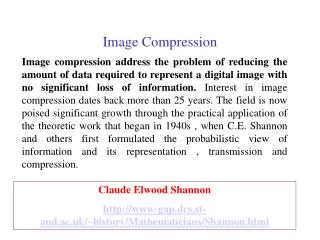
Image Compression
Image Compression. Fundamentals: Coding redundancy The gray level histogram of an image can reveal a great deal of information about the image That probability (frequency) of occurrence of gray level r k is p(r k ),. Image Compression. Fundamentals: Coding redundancy
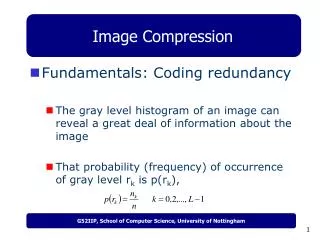

Image Compression
E N D
Presentation Transcript
Image Compression • Fundamentals: Coding redundancy • The gray level histogram of an image can reveal a great deal of information about the image • That probability (frequency) of occurrence of gray level rk is p(rk),
Image Compression • Fundamentals: Coding redundancy • If the number of bits used to represent each value of rk is l(rk), the average number of bits required to represent each pixel is • To code an MxN image requires MNLavg bits
Image Compression • Fundamentals: Coding redundancy • some pixel values more common than others
Image Compression • Fundamentals: Coding redundancy • To code an MxN image requires MNLavg bits • If m-bit natural binary code is used to represent the the gray levels, then
Image Compression • Fundamentals: Coding redundancy • To code an MxN image requires MNLavg bits • If m-bit natural binary code is used to represent the the gray levels, then
Image Compression • Fundamentals: Coding redundancy • Variable length Coding: assign fewer bits to the more probable gray levels than to less probable ones can achieve data compression
Image Compression • Fundamentals: Interpixel (spatial) redundancy • neighboring pixels have similar values • Binary images • Gray scale image (later)
Image Compression • Fundamentals: Interpixel (spatial) redundancy: Binary images • Run-length coding • Mapping the pixels along each scan line into a sequence of pairs (g1, r1), (g2, r2), …, • Where gi is the ith gray level, ri is the run length of ith run
Image Compression • Example: Run-length coding Row 1: (0, 16) Row 2: (0, 16) Row 3: (0, 7) (1, 2) (0, 7) Row 4: (0, 4), (1, 8) (0, 4) Row 5: (0, 3) (1, 2) (0, 6) (1, 3) (0, 2) Row 6: (0,2) (1, 2) (0,8) (1, 2) (0, 2) Row 7: (0, 2) (1,1) (0, 10) (1,1) (0, 2) Row 8: (1, 3) (0, 10) (1,3) Row 9: (1, 3) (0, 10) (1, 3) Row 10: (0,2) (1, 1) (0,10) (1, 1) (0, 2) Row 11: (0, 2) (1, 2) (0, 8) (1, 2) (0, 2) Row 12: (0, 3) (1, 2) (0, 6) (1, 3) (0, 2) Row 13: (0, 4) (1,8) (0, 4) Row 14: (0, 7) (1, 2) (0, 7) Row 15: (0, 16) Row 16: (0, 16) encode decode
Image Compression • Fundamentals: Psychovisual redundancy • some color differences are imperceptible
Image Compression • Fidelity criteria • Root mean square error (erms) and signal to noise ratio (SNR): • Let f(x,y) be the input image, f’(x,y) be reconstructed input image from compressed bit stream, then
Image Compression • Fidelity criteria • erms and SNR are convenient objective measures • Most decompressed images are view by human beings • Subjective evaluation of compressed image quality by human observers are often more appropriate
Image Compression • Fidelity criteria
Image Compression • Image compression models
Image Compression • Exploiting Coding Redundancy • These methods, from information theory, are not limited to images, but apply to any digital information. So we speak of “symbols” instead of “pixel values” and “sources” instead of “images”. • The idea: instead of natural binary code, where each symbol is encoded with a fixed-length code word, exploit nonuniform probabilities of symbols (nonuniform histogram) and use a variable-length code.
Image Compression • Exploiting Coding Redundancy • Entropy • is a measure of the information content of a source. • If source is an independent random variable then you can’t compress to fewer than H bits per symbol. • Assign the more frequent symbols short bit strings and the less frequent symbols longer bit strings. Best compression when redundancy is high (entropy is low, histogram is highly skewed).
Image Compression • Exploiting Coding Redundancy • Two common methods • Huffman coding and, • LZW coding
Image Compression • Exploiting Coding Redundancy • Huffman Coding • Codebook is precomputed and static. • Compute probabilities of each symbol by histogramming source. • Process probabilities to precompute codebook: code(i). • Encode source symbol-by-symbol: symbol(i) -> code(i). • The need to preprocess the source before encoding begins is a disadvantage of Huffman coding
Image Compression • Exploiting Coding Redundancy • Huffman Coding
Image Compression • Exploiting Coding Redundancy • Huffman Coding
Image Compression • Exploiting Coding Redundancy • Huffman Coding • Average length of the code is 2.2.bits/symbol • The entropy of the source is 2.14 bits/symbol
Image Compression • Exploiting Coding Redundancy • Huffman Coding
Image Compression • Exploiting Spatial/Interpixel Redundancy • Predictive Coding • Image pixels are highly correlated (dependent) • Predict the image pixels to be coded from those already coded
Image Compression • Exploiting Spatial/Interpixel Redundancy • Predictive Coding • Differential Pulse-Code Modulation (DPCM) • Simplest form: code the difference between pixels DPCM: 82, 1, 3, 2, -32, -1, 1, 4, -2, -3, -5, …… Original pixels: 82, 83, 86, 88, 56, 55, 56, 60, 58, 55, 50, ……
image histogram (high entropy) DPCM histogram (low entropy) Image Compression • Exploiting Spatial/Interpixel Redundancy • Predictive Coding • Key features: Invertible, and lower entropy (why?)
Image Compression • Exploiting Spatial/Interpixel Redundancy • Higher Order (Pattern) Prediction • Use both 1D and 2D patterns for prediction 1D Causal: 2D Causal: 1D Non-causal: 2D Non-Causal:
Image Compression • Exploiting Spatial/Interpixel Redundancy 2D Causal:
Image Compression • Quantization • Quantization: Widely Used in Lossy Compression • Represent certain image components with fewer bits (compression) • With unavoidable distortions (lossy) • Quantizer Design • Find the best tradeoff between maximal compression minimal distortion
Image Compression • Quantization • Scalar quantization Uniform scalar quantization: 248 8 40 ... 24 1 2 3 4 Non-uniform scalar quantization:
Image Compression • Quantization • Scalar quantization
Image Compression • Quantization • Vector quantization and palletized images (gif format)
Image Compression • Palletized color image (gif) • A true colour image – 24bits/pixel, R – 8 bits, G – 8 bits, B – 8 bits • A gif image - 8bits/pixel 1677216 possible colours 256 possible colours
Image Compression Exploits psychovisual redundancy • Palletized color image (gif) • A true colour image – 24bits/pixel, R – 8 bits, G – 8 bits, B – 8 bits • A gif image - 8bits/pixel 1677216 possible colours 256 possible colours
Image Compression • Palletized color image (gif) (r, g, b) r0 g0 b0 r1 g1 b1 Record the index of that colour (for storage or transmission) To reconstruct the image, place the indexed colour from the Colour Table at the corresponding spatial location For each pixel in the original image Find the closest colour in the Colour Table r255 g255 b255 Colour Table
Image Compression • Palletized color image (gif) (r, g, b) r0 g0 b0 How to choose the colours in the table/pallet? r1 g1 b1 Record the index of that colour (for storage or transmission) To reconstruct the image, place the indexed colour from the Colour Table at the corresponding spatial location For each pixel in the original image Find the closest colour in the Colour Table r255 g255 b255 Colour Table
Image Compression • Construct the pallet (vector quantization, k-means algorithm) B (r, g, b) G A pixel corresponding to A point in the 3 dimensional R, G, B space R
Image Compression • Construct the pallet (vector quantization, k-means algorithm) B G Map all pixels into the R, G, B space, “clouds” of pixels are formed R
B G R Image Compression Group pixels that are close to each other, and replace them by one single colour • Construct the pallet (vector quantization, k-means algorithm)
Image Compression Representative colours placed in the colour table B r0 g0 b0 r1 g1 b1 G r255 g255 b255 Colour Table R
Image Compression • Discrete Cosine Transform (DCT) • 2D-DCT • Inverse 2D-DCT where
Image Compression DC component low frequency high frequency 2D-DCT image block low frequency high frequency DCT block
JPEG Compression 8 x8x blocks - 128 DCT scalar quantization zig-zag scan
JPEG Compression • The Baseline System – Quantization X(u,v): original DCT coefficient X’(u,v): DCT coefficient after quantization Q(u,v): quantization value
JPEG Compression • Why quantization? • to achieve further compression by representing DCT coefficients with no greater precision than is necessary to achieve the desired image quality • Generally, the “high frequency coefficients” has larger quantization values • Quantization makes most coefficients to be zero, it makes the compression system efficient, but it’s the main source that make the system “lossy”
JPEG Compression • Quantization is the step where we actually throw away data. • Luminance and Chrominance Quantization Table • Smaller numbers in the upper left direction • larger numbers in the lower right direction • The performance is close to the optimal condition Quantization Dequantization
JPEG Compression Quantization Dequantization
JPEG Compression • Exploiting Psychovisual Redundancy • Exploit variable sensitivity of humans to colors: • We’re more sensitive to differences between dark intensities than bright ones. • Encode log(intensity) instead of intensity. • We’re more sensitive to high spatial frequencies of green than red or blue. • Sample green at highest spatial frequency, blue at lowest. • We’re more sensitive to differences of intensity in green than red or blue. • Use variable quantization: devote most bits to green, fewest to blue.
JPEG Compression • Exploiting Psychovisual Redundancy • NTSC Video Y bandlimited to 4.2 MHz I to 1.6 MHz Q to .6 MHz
JPEG Compression • Exploiting Psychovisual Redundancy • In JPEG and MPEG Cb and Cr are sub-sampled