Understanding Network Search in Distributed Systems
This overview delves into the analysis of network search methodologies, particularly in the context of web search engines and distributed databases. The document explores how information networks, exemplified by the web, handle vast amounts of data through effective navigation and crawling techniques. It discusses the evolution of web search engines, from simple keyword annotation to advanced metrics like Google’s PageRank. Additionally, it covers distributed databases, emphasizing peer-to-peer networks and the use of Distributed Hash Tables for efficient data retrieval among peers.

Understanding Network Search in Distributed Systems
E N D
Presentation Transcript
TELCOM2125: Network Science and Analysis Konstantinos Pelechrinis Spring 2013 Figures are taken from: M.E.J. Newman, “Networks: An Introduction”
Web search • Information networks store large amounts of data in their vertices • These information is useless unless we find a way to navigate through the network and find the appropriate vertices • Web is on very illustrative example of such an information network • The Web is a directed network, where vertices are the webpages and the edges are the directed links between the pages • Webpages include information and the goal of web search engines is to identify those vertices (i.e., webpages) that include the most relevant information
Web search • The main process that web search involves is crawling • Breadth first search • Many more details for improving performance • Distributed crawling, repeated crawling etc.
Web search • The first generation of web search engines were simply annotating the webpages crawled with keywords found in their text • Various heuristics • Frequency of a term, position on webpage etc. • Modern web search engines make use of network elements as well • Textual annotations are still there • Used as a first step to identify a fairly broad set of also possibly irrelevant with the query web pages • Network metrics are further used to narrow down these sets • Google uses the PageRank centrality metric
Web search • Of course PageRank is only one of the elements in the full search algorithm of Google • One interesting point is that PageRank (and in general any centrality measure that might be used) does not depend on the specific query • Hence, it can be computed offline, accelerating significant the response time • Of course PageRank has disadvantages too • A webpage might have a high PageRank value for a reason unrelated to the current search query
Searching distributed databases • An example of a distributed database is a peer-to-peer network • In a peer-to-peer network participating users have specific files that they store in their machine(s) • Users are logically connected • An edge between two users does not mean that they are physically connected but they have an overlay communication • They are “neighbors” in the network
Searching distributed databases • One could take an approach similar to web search • Central entity that has all the entries “who has what” • Keeping these databases centrally is not a good idea • High load, single point of failure etc. • How can we search in this distributed database? • Simple but naïve approach • Entries are randomly scattered across peers • When a peer wants to query a key sends the query to all the peers • Does not scale (huge traffic/query load and needs to keep track of all the peers)
Superpeers design • Most modern peer-to-peer networks deploy a hierarchical overlay of supernodes • Supernodes are high-bandwidth nodes • Typical clients connect to supernodes • The latter keep track of the files each one of its client has • The entire search is performed at the network of supernodes
Distributed hash tables • Every peer has an n-bit integer identifier in the range of [0, 2n-1] • Every key is an integer in the same range • For this we use hash functions • A hash function maps “names” to integers • in some range. • It is an many to one mapping, so collisions • can occur. E.g., “John Smith” and “Sandra • Dee” map to the same integer.
Distributed hash tables • Recall: peers’ IDs and hashed keys are at the same range • Every entry is being “stored” to the peer whose ID is the closest to the hashed key • Closest is the immediate successor • Example • n = 4 IDs of peers and hashed keys in [0, 15] • Existing peers: 1, 3, 4, 5, 8, 10, 12 and 14 • Key = 13 stored at peer 14 • Key = 15 stored at peer 1
Distributed hash tables • Let us assume that Alice wants to find the database entry for the movie “Die Hard 2” • Alice hashes the key “Die Hard 2” • E.g., h(“Die Hard 2”) = 11 (the hash function is known to all peers!) • How does she find the peer responsible for key 11? • She clearly cannot keep track of all the peers at the system (ID and their IP)
Who’s resp for key 11? I am Circular DHT • Each peer is aware of only immediate successor and predecessor 1 3 15 4 Overlay network Links are not physical links but logical connections. 12 5 10 8 Number of queries grow linearly with the number of peers!!
Circular DHT with shortcuts • With circular DHT each peer keeps track of 2 peers • Fairly large number of queries on average • How can we reduce the number of queries? • Increase the number of peers you keep track of • Tradeoff
Who’s resp for 11? Shortcut example • Messages are reduced from 6 to 3 • Potentially we can have a design where each peer has O(logn) neighbors and there are O(logn) messages exchanged per query 1 3 15 4 12 5 10 8
Message passing • A variation of the distributed search problem is the problem of message passing • How can we get a message to a particular node in the network? • Milgram’s “small-world” experiment • The most stunning thing, is not that the messages that reached the destination followed short paths, but that people were actually able to find them! • If you have a bird’s eye view of the topology you can easily find the shortest path • However, Milgram’s experiment participants did not have this knowledge
Message passing • How did people find these short paths to the target? • Can we come up with an algorithm that will do the job efficiently? • How does the performance of that algorithm depend on the structure of the network? • Preview: Networks need to have a specific structure if we want to solve the above navigation problem
Kleinberg’s model • In Milgram’s experiment, participants were instructed to send the message to an acquaintance that is closer to the target • “Closer” can take many different definitions • There are many dimensions that we can examine connections • E.g., spatial, education status, work etc. • Kleinberg made use of a model similar to the small-world • In particular he considered c=2 • He further defined closeness based on the hop-distances on the ring • Every node is aware of the positions of their acquaintances and of the target node
Kleinberg’s model • He modeled the message passing process through a greedy algorithm • An individual passes the message to his neighbor that is closer to the target node • The message will always reach the destination • Worst case: The message will be passed around the ring • Shortcuts will improve this performance • Kleinberg showed that the greedy algorithm can find the target at O(log2n) steps • This is possible only for a particular arrangement of the shortcuts!
Kleinberg’s model • Instead of assuming that shortcuts are placed uniformly at random between vertices on the ring, shortcuts are more probable to connect vertices that are “closer” on the ring • It is more probable to meet someone that lives in our city as compared to someone that lives in a different state • As in the small-world model we place a shortcut with probability p for every existing edge • Since c=2 there are n edges in total • On average, every node gets 2p shortcut edges
Kleinberg’s model • The difference of this model is on how the ends of the shortcuts are picked • They are still picked uniformly at random but now we first pick the distance r that they will span • r it samples from a probability distribution: Kr-α • K is the normalizing constant, while α is non-negative • For α=0 we have the original small-world model • For α>0 the model shows preference to connections between nearby vertices
Kleinberg’s model • The probability that two vertices at distance r are connected through a shortcut is Kr-α/n • Furthermore, we have np expected shortcut edges • Hence, the expected number of shortcuts between a given pair of vertices at distance r is pKr-α • At the limit of large n this is the probability of a shortcut between a given pair of vertices at distance r • The normalization constant is found by the condition:
Kleinberg’s model • We will show that for a suitable choice of α the greedy algorithm can find the target node quickly • We divide the vertices into different classes based on their distance from the target node • Class 0 target node • Class 1 nodes at distance 2≤d<4 from the target • Class 2 nodes at distance 4≤d<8 from the target • Class k nodes at distance 2k-1≤d<2k from the target • Class k has nk=2k vertices
Kleinberg’s model • Consider that at some point of the greedy algorithm execution the message is at a vertex of class k • How many more steps will it take before the message leaves class k and passes into a lower class? • The total number of vertices in the lower classes is: • The maximum distance between any node in these classes and the vertex at class k that currently has the message is 3x2k-2 < 2k+2
Kleinberg’s model • The probability that the node that currently holds the message has a shortcut at some vertex at lower class is at least: Kp(2k+2)-α • Given that there are at least 2k-1 vertices in lower classes we have that the total probability of having a shortcut at any of the lower class nodes is: (2k-1)Kp(2k+2)-α • We can use the above probability in order to find the expected number of message “passings” within class k before finding a k-class vertex that has the a shortcut to a lower class:
Kleinberg’s model • Since there are log2(n+1) classes in total the upper bound on the expected number of steps l needed to reach the target in the worst case is: • Using the definition for K we have: • When α=1 it is possible to recover the short paths through a greedy algorithm, only knowing our immediate connections
Kleinberg’s model • Hence Kleinberg’s model leaves us with two takeaways • It is possible for the small-world paths can be found distributively • There is only one specific structure of the shortcuts that allows this • Hence, based on this and on Milgram’s seminal experimental results, social networks seem to have a particular structure that makes path finding possible
A hierarchical model • How actual message passing works? • “Reverse small-world” experiment by Killworth and Bernard • Name, occupation and geographic location of the target are the information that lead subjects decide where to forward the message next • If we know the geographic location how would we pass the message? • At each step, we narrow down the search to a smaller geographic area, until we reach an area so small that someone there knows the target directly • E.g., if we are looking for a target in a specific neighborhood in London, we might first sent something at a connection in Europe, this one will forward the message to someone in England and so on
A hierarchical model • This is also the way that Kleinberg’s model works • We divided the circle to classes, which were getting smaller as we were approaching the target vertex • Watts et al. proposed a similar hierarchical model • The interplay between the dimension we consider (e.g., geographic) and the social structure can be captured through a tree • For example, if we consider the geography, the world could be divided in the top level in continents, the continents to countries, the countries to cities, the cities to provinces etc. • Division stops when the units are so small that it can be assumed that everyone knows everyone
A hierarchical model • For simplicity let us assume that the divisions at the dimension we consider are binary • Assume that groups at the tree leaves have the same size g • With n individuals we have n/g groups and log2(n/g) levels • The distance to the target is measured in terms of the tree • Lowest common ancestor in the tree that they share with the traget • Less conservative • Social network is correlated with the hierarchical tree
A hierarchical model • Even though in the model people are less possible to know others that reside “far”, there are also more further individuals as compared to the ones close by • Hence it is quiet possible for an individual to know people both near and far • Consider a case where every node has at least one connection at every “distance” • How would a greedy algorithm work in this case? • It is not very realistic though to assume that each individual knows at least one person at each distance
A hierarchical model • Watts et al. considered a more realistic scenario, where there is a probability pm for two individuals with the lowest common ancestor at level m to be connected • m=0 for groups that are immediately adjacent • m increases by one for each higher level up to a maximum of log2(n/g)-1 • Consider a vertex j. The number of other vertices that share a common ancestor at level m with j is 2mg • Hence, the expected number of connections with these vertices is: 2mgpm=Cg2(1-β)m
A hierarchical model • Summing over all levels, the average degree is: • Which gives a value for C: • C dictates the number of connections that each individual has • For large n we get:
A hierarchical model • Now consider the greedy forwarding again • If a vertex wants to pass a message to the opposite sub-tree at level m he can do so given that he has an appropriate connection • This happens with probability Cg2(1-β)m • If such a connection does not exist, he can pass it to another vertex at his sub-tree and the process is repeated • The expected number of “local message passings” before a neighbor in the opposite sub-tree is found is: 2(β-1)m/Cg • Then the total expected number of steps to reach the target is:
A hierarchical model • Of course we have assumed that the vertex that currently has the message either has a connection at his own sub-tree or one at the opposite sub-tree • This is not necessary to hold true • The vertex can have connections only further from the target • Target is not found • Failures in Milgram’s experiment • However, when the target is found the previous equations gives an estimate of the number of steps needed • At the limit of large n:
A hierarchical model • Again we see that we can find the shortest path through a greedy, fully distributed, algorithm only if β=1 • Both results (Kleinberg’s model and hierarchical model) are still not yet fully understood • It is possible that the models miss some important feature that makes message passing robust in real worlds • People might have a better process as compared to greedy forwarding • It might also be possible that the models are precise and the world is really tuned as the models require for finding the short paths (α=1 or β=1)
Discussion of the message passing models • Kleinberg’s model really showed that networks can be searchable through simple greedy processes • However, the model itself is not representative of real world (social) networks • In particular, Kleinberg’s model is built on top of a geometric lattice • Geometry is implicitly assumed to be a social proxy • Closeness on the lattice translates to closeness in the social space • Watts et al. model is built on the fact that people in the social plane can have multiple identities
Discussion of the message passing models • Two specific people can be close in the one dimension (e.g., live in the same neighborhood) but far in the other (e.g., do completely different occupations) www.sciencemag.org SCIENCE VOL 296 MAY 2002
Discussion of the message passing models • Considering more than one dimensions while searching can help distributed search tremendously • The class of networks that are searchable is becoming larger www.sciencemag.org SCIENCE VOL 296 MAY 2002