ECMWF/EUMETSAT NWP-SAF Satellite data assimilation Training Course

1. ECMWF/EUMETSAT NWP-SAF Satellite data assimilation Training Course 1 to 4 July 2013

2. ECMWF/EUMETSAT NWP-SAF Satellite data assimilation Training Course The detection and assimilation of clouds in IR radiances

3. Task 1: Overlay clear and cloudy Tropical IASI spectra • Duplicate Tropical profile ( tropic.nc > copy_1_tropic.nc) • Analyse copy_1_tropic.nc change cloud parameters (2D) • Edit / visualise IASI SPECTRUM (with tropic.nc ) • Edit / drop IASI SPECTRUM (with copy_1_tropic.nc)

4. Task 1: Overlay clear and cloudy Tropical IASI spectra

5. Option 1:Detect and reject cloud contaminated observationsOption 2:Explicitly estimate cloud parameters from the radiances within the data assimilation (simultaneously with T,Q,O3 etc..)

6. Option 1:Detectand rejectcloud contaminated observationsOption 2:Explicitly estimate cloud parameters from the radiances within the data assimilation (simultaneously with T,Q,O3 etc..)

7. Cloud detection methods • Simple window channel departure checks • Co-located imager checks • Pattern recognition algorithms • Hybrid systems

8. Cloud detection methods • Simple window channel departure checks • Co-located imager checks • Pattern recognition algorithms • Hybrid systems

9. Window channels have the highest sensitivity to cloud

10. Observed radiance at 11 um minus radiance calculated from background in clear sky Clear population Cold departures indicating cloud contamination in OBS

11. Yobs – H(Xclear) > dTthreshold

12. …results in a asymmetric population surviving the check …!

13. Cloud detection methods • Simple window channel departure checks • Co-located imager checks • Pattern recognition algorithms • Hybrid systems

14. IASI field of view AVHRR imager pixels

15. Homogenous clear Homogenous cloudy Mixed cloud scene

16. Scatter stdv versus mean Tb AVHRR standard deviation 220K 250K 280K 300K AVHRR mean radiance

17. Homogenous clear AVHRR standard deviation 220K 250K 280K 300K AVHRR mean radiance

18. Homogenous cloudy AVHRR standard deviation 220K 250K 280K 300K AVHRR mean radiance

19. Mixed scene AVHRR standard deviation 220K 250K 280K 300K AVHRR mean radiance

20. Cloud detection methods • Simple window channel departure checks • Co-located imager checks • Pattern recognition algorithms • Hybrid systems

21. Zoom in …

22. Clear spectrum Cloudy spectrum

23. Break point

24. Break point depends on cloud height Zero Cloud Cloud at 500hPa Cloud at 400hPa Cloud at 200hPa

25. First filter and find the break point Observed spectrum minus clear sky computed spectrum observed-calculated (K) Vertically ranked channel index

26. First filter and find the break point Observed spectrum minus clear sky computed spectrum observed-calculated (K) Vertically ranked channel index

27. Break point Channels retained Channels rejected observed-calculated (K) Vertically ranked channel index

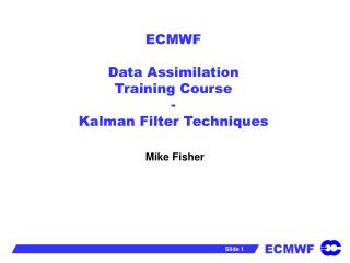
28. AIRS channel 226 at 13.5micron (peak about 600hPa) unaffected channels assimilated CLOUD pressure (hPa) contaminated channels rejected AIRS channel 787 at 11.0 micron (surface sensing window channel) temperature jacobian (K)

29. Cloud detection methods • Simple window channel departure checks • Co-located imager checks • Pattern recognition algorithms • Hybrid systems

30. Why do we need Hybrid systems ? • Yobs – H(Xclear) > dT • But sometimes large errors in the background can lead to: • False rejection of a good observation • Missed rejection of a bad observation

31. Option 1:Screen the radiance data and reject cloud/rain contaminated observationsOption 2:Explicitly estimate cloud parameters from the radiances within the data assimilation (simultaneously with T,Q,O3 etc..)

32. It looks very difficult …why would we try to do this ?

33. We have to throw away lots of data !!! AIRS channel 226 at 13.5micron (peak about 600hPa) unaffected channels assimilated CLOUD pressure (hPa) contaminated channels rejected AIRS channel 787 at 11.0 micron (surface sensing window channel) temperature jacobian (K)

34. Sensitive areas and cloud cover Location of sensitive regions Summer-2001 (no clouds) sensitivity surviving high cloud cover monthly mean high cloud cover sensitivity surviving low cloud cover monthly mean low cloud cover From McNally (2002) QJRMS 128

35. …so what is required to do this ?

36. The cost function J(X) background error covariance model state observations observation operator (maps the model state to the observation space) observation* error covariance If we wish to assimilate cloudy radiance observations …..

37. The cost function J(X) model state must include clouds (clw,cic,cf)

38. Two approaches to assimilate cloud affected infrared radiances • Simplified system: • very simple cloud representation • currently limited to overcast scenes • no information on clouds taken from model • no back interaction with model via physics X=(T,Q,V,cp,cf) cp cf • Advanced system: • very complex cloud representation • all cloud conditions treated • information on clouds taken from model • back interaction with model via physics X=(T,Q,V,ciw,clw,cc)

39. The cost function J(X) Background error covariance must include clouds (clw,cic,cf)

40. The cost function J(X) Obervations operator (RT and Model) must include clouds (clw,cic,cf)

41. Potential difficulties • The cloud uncertainty in radiance terms may be an order of magnitude larger than the T and Q signal (i.e. 10s of kelvin compared to 0.1s of kelvin) • The radiance response to cloud changes is highly non-linear (i.e. H(x) = Hx(x)) • Errors in background cloud parameters provided by the NWP system may be difficult to quantify and model • Conflict between having enough cloud variables for an accurate RT calculation while limiting the number of cloud variables to those that can be uniquely estimated in the analysis from the observations

42. Observed radiance at 11 um minus radiance calculated from background in clear sky Clear population Cold departures indicating cloud contamination in OBS

43. Potential difficulties • The cloud uncertainty may be an order of magnitude larger than the T and Q signal (i.e. 10s of kelvin compared to 0.1s of kelvin) • The radiance response to cloud changes is highly non-linear (i.e. H(x) = Hx(x)) • Errors in background cloud parameters provided by the NWP system may be difficult to quantify and model • Conflict between having enough cloud variables for an accurate RT calculation while limiting the number of cloud variables to those that can be uniquely estimated in the analysis from the observations

44. Clear and Cloudy Jacobians(impact at the cloud top) dR/dT500 = 0 dR/dT* = 1 dR/dT500 = 1 dR/dT* = 0 full cloud at 500hPa surface surface

45. Potential difficulties • The cloud uncertainty may be an order of magnitude larger than the T and Q signal (i.e. 10s of kelvin compared to 0.1s of kelvin) • The radiance response to cloud changes is highly non-linear (i.e. H(x) = Hx(x)) • Errors in background cloud parameters provided by the NWP system may be difficult to quantify and model • Conflict between having enough cloud variables for an accurate RT calculation while limiting the number of cloud variables to those that can be uniquely estimated in the analysis from the observations

46. Observed radiance at 11 microns minus radiance calculated from NWP cloud background profile Many clouds with significant radiance signals are accurately represented by the NWP model and RT modelled !

47. Potential difficulties • The cloud uncertainty may be an order of magnitude larger than the T and Q signal (i.e. 10s of kelvin compared to 0.1s of kelvin) • The radiance response to cloud changes is highly non-linear (i.e. H(x) = Hx(x)) • Errors in background cloud parameters provided by the NWP system may be difficult to quantify and model • Conflict between having enough cloud variables for an accurate RT calculation while limiting the number of cloud variables to those that can be uniquely estimated in the analysis from the observations

48. T n T P P n Choice of cloud parameters and ambiguity with T and Q A very simple cloud model (e.g. single layer grey cloud amount and pressure) should more readily estimated from the data (independently of T and Q), but will make the forward RT calculation very inaccurate in many cloud conditions A more complex cloud model (e.g. cloud liquid and ice at each model level) will allow a more forward RT calculation, but may be difficult to estimate independently of T and Q and may alias into erroneous increments

49. Two approaches to assimilate cloud affected infrared radiances

50. Two approaches to assimilate cloud affected infrared radiances • Simplified system: • very simple cloud representation • currently limited to overcast scenes • no information on clouds taken from model • no back interaction with model via physics X=(T,Q,V,cp,cf) cp cf • Advanced system: • very complex cloud representation • all cloud conditions treated • information on clouds taken from model • back interaction with model via physics X=(T,Q,V,ciw,clw,cc)