Download
1 / 49
561 likes | 1.17k Views
Chapter 2 Fermat’s Principle and Its Applications. A. S. P. B. S . 2.1 Introduction. Geometrical optics 幾何光學: The field of optics under ray approximation ( 0).

E N D
Chapter 2 Fermat’s Principle and Its Applications
A S P B S 2.1 Introduction Geometrical optics幾何光學:The field of optics under ray approximation ( 0) Fermat’s Principle:the ray will correspond to that path for which the time taken is an extremum in comparison to the nearby path. Fig. 2.1 The light emitted by the point source P is allowed to pass through a circular hole and if the diameter of the hole is very large compared to the wavelength of light then the light patch on the screen SS has well defined boundaries.
B ds C C A Let n(x, y, z) is the position dependent refractive index.The time taken to traverse path ds is Fig. 2.2 If the path ACB represents the actual ray path then the time taken in traversing the path ACB will be an extremum in comparison to any nearby path ACB. According to Fermat’s principle
B E C D A Fig. 2.3 Since the shortest distance between two points is along a straight line, light rays in a homogeneous medium are straight lines; all nearby paths like AEB or ADB will take longer times.
S A B R N M Q P A 2.2 Laws of Reflection and Refraction from Fermat’s Principle Reflection APS = SPB Fig. 2.4 The shortest path connecting the two points A and B via the mirror is along the path APB where the point P is such that AP, PS and PB are in the same plane and APS = SPB; PS being the normal to the plane of the mirror. The straight line path AB is also a ray.
A 1 h1 1 L x n1 N M Q P R n2 x 2 h2 2 B L The optical path length from A to B is Snell’s law of refraction n1sin1 = n2sin2 Fig. 2.5 A and B are two points in media of refractive indices n1 and n2. The ray path connecting A and B will be such that n1 sin 1 = n2 sin 2 .
A Q L P Q ¢ L S C B Example 2.1 Consider a set of rays, parallel to the axis, incident on a paraboloidal reflector. Show that all the rays will pass through the focus of the paraboloid. PQ’ + Q’S = PQ’ + Q’L’ Fig. 2.6 All rays parallel to the axis of a paraboloidal reflector pass through the focus after reflection (the line ACB is the directrix). It is for this reason that antennas (for collecting electromagnetic waves) or solar collectors are often paraboloidal in shape.
P S2 S1 Q Fig. 2.7 All rays emanating from one of the foci of an ellipsoidal reflector will pass through the other focus.
S n2 n1 P C O Q I r x y0 y M Example 2.3 Consider a spherical refracting surface SPM separating two media of refractive indices n1 and n2. The point C represents the center of SPM. Consider two points O and Q such that the points O, C and Q are in a straight line. Use Fermat’s principle to find the ray connecting O and Q. Fig. 2.8 SPM is a spherical refracting surface separating two media of refractive indices n1 and n2. C represents the center of the spherical surface.
若很小 同理
則有y = y0滿足 上式之結果是在假設很小下所得之近似,即近軸近似paraxial approximation。 若以P為原點,左方為負,右方為正,上式可一般化為
n1 P S O I n2 考慮光自物點 O 經球面 S 處折射至 P 點,若軸上 I 點為軸上一點使得n1OS n2SI與 S無關,證明 n1OS n2SI為極值且與 無關。 Fig. 2.9 : The refracted ray is assumed to diverge away from the principal axis. 假設 O 經球面 S 處至 P 的路徑,則有 需為極值。 其中等號右方第一項與S 無關,若Lop為極值,則右方第二項必為極值。因此IS、SP必成直線。如此,光折射至介質2中看起來像是由 I 射出。因此虛像 I 滿足的條件為 n1OS n2SI為極值。
x ds 因此可定義一不變量(invariant)在整個光路上均不變。 dx dz 若最初光折射率為n1處與z軸夾角為1,則 n4 4 x z 3 n3 3 2 n2 1 n1 1 z 2.3 Ray Paths in an Inhomogeneous Medium 非均質介質可考慮成由一層層很薄折射率不同的均勻介質所組成。在層與層間的介面光線進出的角度滿足Snell‘s law,即 在整個光行進過程中,此值保持不變。因此當介質中折射率變化時, 角便隨之改變,光路便逐漸彎曲。
在氣壓固定下, 考慮在熱天時,地面溫度較高。此時空氣折射率在較接近地面處較低。此時折射率的變化可近似的表視為 其中x為距地面的高度,n0為地面x = 0處之折射率 考慮一光線在x = 0處方向為水平,假若在眼睛位置E處,折射率為 ne且光與水平夾角為e。則有 若e << 1,則 or
x(m) C P E W W B B R1 R2 M z (m) 在一典型的熱天中,地表近路面處溫度T0 323 K (50 C),離地面1.5 m處溫度Te 303 K (30 C), x1 = 1.5 m, n0 = 1.00026 and k = 1.234105 m1
R x(m) C E P R2 R1 M 1.10 1.05 1.00 n(x) z (m) P = 0.43 m Fig. 2.12 Ray paths in a medium characterized by Eqs. (21) and (22). The object point is at a height of 1/( 0.43m) and the curves correspond to 1 = + /10, 0, -/60, -/30, -/15 and -/10. The shading shows that the refractive index increases with x.
若上圖中有一道光在x = 0.2 m處成為水平,則其在P點發射時與z軸之夾角1滿足 n(0.43) = 1.06420, n(0.2) = 1.03827
C 3 3 3 3 3 3 3 3 E C E P x (m) R1 R1 2 2 2 2 2 2 2 2 1 1 1 1 1 1 1 1 M R2 M R2 0 0 0 0 0 0 0 0 0 0 0 0 0 0 0 0 5 5 5 5 5 5 5 5 10 10 10 10 10 10 10 10 15 15 15 15 15 15 15 15 20 20 20 20 20 20 20 20 1.10 1.00 1.05 n z (m) P P = 2.8 m Fig. 2.13 Ray paths in a medium characterized by Eqs. (21) and (22). The object point is at a height of 2.8m and the curves correspond to 1 (the initial launch angle) = 0, -/60, -/30, -/16 , -/11 , -/10 and -/8. The shading shows that the refractive index increases with x.
此道光成為水平方向時折射率滿足 若上圖中物體位於 x = 2.8 m,此處 n(x) 1.1,對一道光以1 = /8
P x (m) E P 1.00 1.10 1.05 z (m) n(x) 另一方面,若折射率隨高度增加而減少,如再冰冷海域,水面溫度遠較上方的空氣低。此時折射率的變化可以下式表示: Fig. 2.14 Ray paths corresponding to the refractive index distribution given by Eq.(23) for an object at a height of 0.5 m; the values of n0, n2 and are given by Eq. (22).
S’ EARTH S Fig. 2.15 The non circular shape of the setting sun. Fig. 2.16 Because of refraction, light from S appears to come from S.
x ds 在一折射率連續變化介質中行進的光線,在其光路上保持不變。光路上一小段路徑長ds有 dx dz z 2.4 The Ray Equation and Its Solutions 在此我們將利用ray equation,討論其非均質介質中所得之解所呈現的光跡。為簡化過程,假設折射率只沿一個方向(x方向)呈連續變化。 將左式等號兩邊各對z微分
or Example 2.7若介質為均勻,即n(x)為常數,則有 直線
Example 2.8若介質為折射率變化為 n(x) = n0 + kx or Assume at z = 0, the ray is launched at x = x1 making an angle 1 with z axis where n1 = n0 + kx1
Consider a parabolic index medium From where let x = x0 sin , and choose the ray is launched at z = 0
In an optical waveguide the refractive medium index distribution is usually in the form thus In a typical parabolic index fiber,
1 = 20 Cladding 0.02 0 0.02 0.02 0.02 0.02 0.02 .02 x (m) Core 1 = 8.13 0 1 = 4 zp -0.02 - - - - - - 0.02 0.02 0.02 0.02 0.02 0.02 1 0 z (mm) z0 = 0 Fig.2.17 Typical ray paths in a parabolic index medium for parameters given by Eq.(33) for 1=4, 8.13 and 20.
20 x (m) L M Q P -20 0 1 zp z (mm) Fig.2.18 Paraxial ray paths in a square law medium. Notice the periodic focussing and defocussing of the beam.
Example 2.10 Obtain the ray equation for refractive index given by From or where Let Since x = x1 at z = 0
Transit Time Calculations in a Parabolic Index Waveguide the ray path inside the core is given by where 光線行進一段長度ds需時
since 當光線沿z軸前進 若z很大時
For a parabolic index waveguide, the broadening will be given by since For the fiber parameters
Reflection from the Ionosphere 太陽輻射之紫外光會將大氣中的氣體分子游離成帶電離子構成所謂之ionosphere(電離層)。此離子化現象在60 km以下高度可忽略。由於在電離層中存在自由電子,折射率可由下式表示(參見chapter 6) Ne(x) 為電子濃度 no./m3 x 為距地面高度 為電磁波之角頻率 q 為電子電量 m 為電子質量 0 為真空容電率 在60 km以上高度,折射率會因電子濃度增加而遞減。
F region 180 km 11 - 3 » ´ ( ) 4 10 m N e max 11 - 3 » ´ ( ) 2.6 10 m N e max 100 km T E region q 1 A B Fig. 2.20 Reflection from the E region of the ionosphere. The point T represents the turning point. The shading shows the variation of the electron density.
Equivalent height (km) Frequency of the exploring waves in MHz Fig. 2.21 Frequency dependence of the equivalent height of reflection from the E and F regions of the ionosphere.
Example 2.9若介質為折射率變化為 考慮一光線由原點入射 where
n1 = 1.5, g = 0.1 m1 Fig. 2.19 Parabolic ray paths (corresponding to 1 = 20, 30,45 and 60)in a medium characterized by linear refractive index variation in the region x > 0 [see Eq.(29)]. The ray paths in the region x < 0 are straight lines.
A n1 h1 i x I P II L - x h2 Optic Axis B Q c / ne c / no Fig. 2.22 The direction of the refracted extraordinary ray when the optic axis (of the uniaxial crystal) is normal to the surface.
A x h1 i I n1 P S2 S1 n() II L - x r h2 B Optic axis Q L Fig. 2.23 The direction of the refracted extraordinary ray when the optic axis (of the uniaxial crystal) lies in the plane of incidence making an angle with the normal to the interface.
I II Optic axis Fig. 2.24 For normal incidence, in general, the refracted extraordinary ray undergoes finite deviation. However, the ray proceeds undeviated when the optic axis is parallel or normal to the surface.
S C Q O θ P x r y M Fig. 2.25 Paraxial image formation by a concave mirror.
S P O Q C y x r M Fig. 2.26 Paraxial image formation by a convex mirror.
n1 n2 S Q O C P r y x M Fig. 2.27 Paraxial image formation by a concave refracting surface SPM.
n1 Q B n2 C C O A Fig. 2.28 All rays parallel to the major axis of the ellipsoid of revolution will focus to one of the focal points of the ellipse provided the eccentricity = n1/n2.
O R P1 P2 C Fig. 2.29 A spherical reflector.
n1 S n2 P I O C d1 r d2 Fig. 2.30 All rays emanating from O and getting refracted by the spherical surface SPM appear to come from I.
S P O I M Fig. 2.31 The Cartesian oval. All rays emanating from O and getting refracted by SPM pass through I.
3 3 3 3 3 3 3 2 2 2 2 2 2 2 1 1 1 1 1 1 1 (mm) x 0 0 0 0 0 0 0 - - - - - - - 1 1 1 1 1 1 1 - - - - - - - 2 2 2 2 2 2 2 - - - - - - - 3 3 3 3 3 3 3 0 0 0 0 0 0 0 2 2 2 2 2 2 2 4 4 4 4 4 4 4 6 6 6 6 6 6 6 8 8 8 8 8 8 8 10 10 10 10 10 10 10 12 12 12 12 12 12 12 (mm) z Fig. 2.32 Ray paths in a graded index medium characterized by Eq. (100).