Download

1 / 18
220 likes | 684 Views
5.4 Runge-Kutta 4 Method. Carl Runge (1856-1927). Martin Wilhelm Kutta (1 867-1944 ). Motivation. With Euler’s method, error is described by a straight line: i.e., it is proportionate to (linear in) D t . We say that error is O( D t ) : “Order D t”, or “Big-O D t ” Can we do better?.

E N D
Carl Runge(1856-1927) Martin Wilhelm Kutta(1867-1944)
Motivation • With Euler’s method, error is described by a straight line: i.e., it is proportionate to (linear in) Dt. • We say that error is O(Dt) : “Order Dt”, or “Big-O Dt” • Can we do better?
First Estimate ∂1 ∂1 = 80 ∆t = 8 • Recall update rule from Euler’s Method: Pn← Pn-1 + f(tn-1, Pn-1) ∆t where f is the derivative function • We call f(tn-1, Pn-1) = 80 the first estimate, or ∂1
Second Estimate ∂2 • Second estimate ∂2 uses the halfway point along the line segment to ∂1
Second Estimate ∂2 ∂2= 112 ∆t = 8 • Combined with slope 0.10 (from dP/dt = 0.10P), this gives us a new endpoint = (0.1)(140)(8) = 112, which is the second estimate∂2. • ∂2 = f(tn-1+0.5t, Pn-1+0.5∂1) t
Third Estimate ∂3 • Third estimate ∂3 uses the halfway point along the line segment from ∂2 • ∂3 =(0.1)(156)(8) = 124.8
Third Estimate ∂3 ∂3= 124.8 • (0.1)(156)(8) = 124.8, which is the third estimate∂3. • ∂3 = f(tn-1+0.5t, Pn-1+0.5∂2) t
Fourth Estimate ∂4 • Fourth estimate ∂4 is taken at end of interval • ∂4 =(0.1)(224.8)(8) = 179.84
Fourth Estimate ∂4 ∂4= 179.8 • ∂4 =(0.1)(224.8)(8) = 179.84, which is the fourth estimate∂4. • ∂4 = f(tn-1+ t, Pn-1+∂3) t
Runge-Kutta 4 Estimate • Bring it all together: a weighted average that privileges the middle values: Pn = Pn-1 + (∂1 + 2∂2 + 2∂3 +∂4) / 6 = 100 + (80 + 2*112 + 2*124.8 + 179.84) / 6 = 222.24 • Relative error = |222.4 - 222.55| / |222.55| = 0.14% (Compare 19% for Euler’s Method) • RK4 error is O(Dt4) : a very small number, because error is < 1.
Runge-Kutta 4 Algorithm t ← t0 P(t0)← P0 Initialize NumberOfSteps for n going from 1 to NumberOfSteps do the following: tn← t0+ n∆t ∂1= f(tn-1, Pn-1) ∂2 = f(tn-1+0.5t, Pn-1+0.5∂1) t ∂3 = f(tn-1+0.5t, Pn-1+0.5∂2) t ∂4 = f(tn-1+ t, Pn-1+∂3) t