Download
1 / 57
670 likes | 983 Views
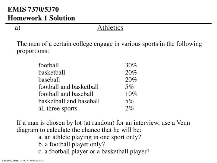
a). Athletics The men of a certain college engage in various sports in the following proportions: football 30% basketball 20% baseball 20% football and basketball 5% football and baseball 10% basketball and baseball 5% all three sports 2%

E N D
a) Athletics The men of a certain college engage in various sports in the following proportions: football 30% basketball 20% baseball 20% football and basketball 5% football and baseball 10% basketball and baseball 5% all three sports 2% If a man is chosen by lot (at random) for an interview, use a Venn diagram to calculate the chance that he will be: a. an athlete playing in one sport only? b. a football player only? c. a football player or a basketball player?
Athletics If an athlete is chosen by lot ( at random), what is the chance that he will be: d. a football player only e. a football player or a baseball player Show details of your approach and solution.
Basketball Football 0.17 0.03 0.12 0.02 0.08 0.03 0.07 S Baseball First construct a diagram as follows:
a. P(one sport only) = P(football only) + P(basketball only) + P(baseball only) = 0.17 + 0.12 + 0.07 = 0.36 b. P(football only) = 0.17 Another approach is: P(F only) = P(F) - P(FBB) - P(FBK) + P(FBBBK) = 0.3 - 0.1 - 0.5 + 0.02 = 0.17
c. P(football or basketball) = 0.17 + 0.12 + 0.03 + 0.08 + 0.02 + 0.03 = 0.45 P(athlete) = P(at least one sport) = 0.17 + 0.12 + 0.03 + 0.08 + 0.02 + 0.03 + 0.07 = 0.52 d. P(football only|athlete) = 0.17/0.52 = 0.3269 e. P(football or baseball|athlete) = 0.40/0.52 = 0.7692
Component Inspection Each day, Monday through Friday, a batch of items sent by a first supplier arrives at a certain inspection facility. Two days a week, a batch also arrives from a supplier. Eighty percent of all supplier 1’s batches pass inspection, and 90% of supplier 2’s do likewise. What is the probability that, on a randomly selected day, two batches pass inspection?
Visualize the process and construct a tree diagram as follows: Probability 0.480 0.120 0.288 0.032 0.072 0.008 1.000 Outcome B B B1B2 B1B2 B1B2 B1B2 Passes 0.8 1 Batch 0.2 Fails 0.6 0.9 2nd Passes 0.4 1st Passes 0.8 0.1 2nd Fails 2 Batches 2nd Passes 0.2 0.9 1st Fails 0.1 2nd Fails Sample Space
P(Two batches pass inspection) = P(Two received Both Pass) = P(Two received) x P(Both pass|Two received) = (0.4) [(0.8)(0.9)] = 0.288
a) JC Nickel The J.C. Nickel department store is considering adopting a new credit management policy in an attempt to reduce the number of credit customers defaulting on their payments. The credit manager has suggested that, in the future, credit should be discontinued to any customer who has twice been a week or more late with his monthly installment payment. He supports his claim by noting that past credit records show that 90% of all those defaulting on their payments were late with at least 2 monthly payments. Suppose from our own investigation we have found that 2% of all credit customers actually default on their payments, and that 45% of those who have not defaulted have had at least 2 late monthly payments. Find the probability that a customer with 2 or more late payments will actually default on his payments and, in light of this probability, analyze the manager’s credit plan in terms of impact on customers.
Let L = late, L = not late, D = default, D = not default, Then after visualization, construct a diagram of the process as follows: Problem a) Outcome Probability DL 0.018 DL 0.002 DL 0.441 DL 0.539 L 0.9 D 0.02 L 0.1 L 0.45 0.98 D 0.55 L 1.0
Problem a) We want to find the probability of default, given that a customer has 2 or more late payments, i.e., Since L = (DL) (DL), And DL=D∩L and DL=D∩L are mutually exclusive events, so that P(L) = P(DL) + P(DL) From the tree diagram P(DL) = 0.018, and P(L) = 0.018 + 0.441 = 0.459
b) Company Bid A company is bidding on three contracts with values of $20 million, $80 million and $50 million with corresponding win probabilities of 1/2, 1/4, and 3/4. Determine and plot the probability mass function and probability distribution function of the contract award amount (in millions of dollars). What is the probability of being awarded at least $100 million? What is the mean, variance & standard deviation of contract award amount (in millions of dollars)?
Problem b) Let C1 = contract 1 was won C1´ = contract 1 was not won C2 = contract 2 was won C2´ = contract 2 was not won C3 = contract 3 was won C3´ = contract 3 was not won P(C1) = 0.50 P(C1´) = 0.25 P(C2) = 0.25 P(C2´) = 0.75 P(C3) = 0.75 P(C3´) = 0.25 X = Value of contracts won (in millions of $)
C3 0.75 C3’ 0.25 C2 0.25 C2’ 0.75 C3 0.75 C1 0.5 C3’ 0.25 C1’ C3 0.75 0.5 C2 C3’ 0.25 0.25 C2’ 0.75 C3 0.75 C3’ 0.25 Problem b) Outcome Probability X C1C2C3 0.09375 150 C1C2C3’ 0.03125 100 C1C2’C3 0.28125 70 C1C2’C3’ 0.09375 20 C1’C2C3 0.09375 130 C1’C2C3’ 0.03125’ 80 C1’C2’C3 0.28125 50 C1’C2’C3’ 0.09375 0 1.0
Problem b) Probability mass and distribution functions of the contract award amount.
Problem b) Probability of being awarded at least $150M: Mean award amount : Variance of award amount : Standard Deviation of Award amount:
12 inch bar A 12 inch bar that is clamped at both ends is to be subjected to an increasing amount of stress until it snaps. Let Y = the distance from the left end at which the break occurs and suppose Y has a probability density function Find the following: 1). The cumulative probability distribution function 2). P (Y 4), P (Y > 6), and P (4 Y 6) 3). E (Y) and the standard deviation of Y 4). The probability that the break point occurs more than 2 inches from the expected breakpoint. 5). The expected length of the shorter segment when the break occurs. , and 0 otherwise
Problem a) Y = distance from left end at which the break occurs 0 y 12 otherwise 12 inches
1). Problem a)
Problem a) for y < 0 0 ≤ y ≤ 12 for y > 12
Problem a) 2).
3). Problem a)
Problem a) Or, since the probability density function is symmetric about 6, the mean of Y is 6
4). Problem a)
Problem a) 5). Let X1 be the shorter piece and X2 be the longer. Then X1 + X2 = 12 and X2 = 12 - X1 Since f(y) is symmetric about = 6, the probability density function of X1 is 0 x1 6 Then
The mean external diameter of a shaft is S = 1.048 inches and the standard deviation is S = 0.0050 inches. The mean inside diameter of the mating bearing is b = 1.063 inches and the standard deviation is b = 0.0025 inches. Assume that both diameters are normally and independently distributed. Bearing/Shaft Analysis
Bearing/Shaft Analysis (a) What is the required clearance, C, such that the probability of an assembly having a clearance less than C is 1/100? (b) What is the probability of interference? (c) What do you recommend to change the probability of interference to 1/1000?
Bearing Xb Shaft XS Bearing/Shaft Analysis - Solution fs(x) fb(x)
D = xb-xs = Clearance of bearing inside diameter minus shaft outside diameter D = b - S = 0.015 D = (b2 + S2)1/2 = 0.00559 so D~N(0.015,0.00559) Bearing/Shaft Analysis - Solution fD(x) d=xb-xs
(a) Find c such that P(D < c) = From the normal table, the Z = -2.33 Then and since Bearing/Shaft Analysis - Solution
(b) Find the probability of interference, i.e., P(D<0) Then Bearing/Shaft Analysis - Solution
(c) To change the probability of interference to 1/1000, there are three choices: 1. Change m 2. Change s 3. Change both m and s Usually, s is changed. In this case Bearing/Shaft Analysis - Solution
30 Contracts Thirty closed-out contracts are selected at random to determine the performance of each. The results are expressed in percent profit (a negative value indicates a loss) as follows: (a) Describe these data in terms of the sample mean, median, range, variance, and standard deviation and graphical techniques including time series, Box Plot, stem-and-leaf plot, histogram, and relative frequency distribution.
30 Contracts (b) Select an appropriate probability distribution using probability plotting as a basis for your selection. (c) If the percent profit has a normal probability distribution, i. Estimate the population mean and standard deviation profit margin in terms of point estimates and 90% confidence intervals. ii. Estimate the probability that a contract will result in a loss. Assess the possible error in your estimate in terms of a 90% confidence interval.
30 Contracts - Solution Time Series of Closed-out Contracts Profit (%) order obtained
30 Contracts - Solution (a) Summary of Descriptive Statistics
The following charts show another construction for Relative Frequency Distribution and Box plot x -4.5 0 9.0 4.5 13.5 18 22.5 Box Plot 20 10 0 -10 18.1 11.7 6.95 3.45 -4.2