Download
1 / 15
150 likes | 294 Views
Logic Synthesis in IC Design and Associated Tools Review-I. Wang Jiang Chau Grupo de Projeto de Sistemas Eletrônicos e Software Aplicado Laboratório de Microeletrônica – LME Depto . Sistemas Eletrônicos Universidade de São Paulo. Computational Problems and Intractability.

E N D
Logic Synthesis in IC Design and Associated Tools Review-I Wang Jiang Chau Grupo de Projeto de Sistemas Eletrônicos e Software Aplicado Laboratório de Microeletrônica – LME Depto. SistemasEletrônicos Universidade de São Paulo
Computational Problems and Intractability SEVERAL Algorithms (efficiency, sometimes also complexity) ONE Problem (complexity) • ALGORITHMS (algorithmics !!): when an algorithm is efficient? • Algorithm is a step-by-step procedure . • Algorithm is different from program .
P2: 4 5 3 7 2 6 P1: 5 4 3 7 2 6 P1: 54 3 7 26(pivot=5) P1: 5 4 3 726(pivot=5) P1: 5 4 3 2 7 6(pivot=5) P3: 3 4 5 7 2 6 P2: 4 3 5 7 2 6 P4: 3 4 5 7 2 6 P2: 2 4 3 5 76 (pivot=2) (pivot=7) P2: 243 5 76 (pivot=2) (pivot=7) P5: 2 3 4 5 7 6 P4: 3 4 5 2 7 6 P4: 3 2 4 5 7 6 P4: 3 4 2 5 7 6 P5: 2 3 4 5 6 7 The (Increasing) Sorting Problem 5 4 3 7 2 6 Insertion Sort Quick Sort P1: 4 5 3 7 2 6 P1: 5 4 3 7 2 6 P1: 5 4 3 7 2 6 P1: 5 4 3 7 2 6 (pivot=5) P1: 5 4 3 7 26(pivot=5) P1: 5 4 3 726(pivot=5) P1: 5 4 3 2 7 6(pivot=5) P1: 2 4 3 5 7 6 (pivot=5) P2: 3 4 5 7 2 6 P2: 2 4 3 5 76 (pivot=2) (pivot=7) P2: 2 4 3 5 6 7 P2: 2 4 3 5 7 6 (pivot=2) P3: 3 4 5 7 2 6 P4: 2 3 4 5 7 6 P3: 2 34 5 6 7 P3: 2 43 5 6 7 P3: 2 43 5 6 7 (pivot=4) P5: 2 3 4 5 6 7
Which Algorithm to Use? • Empirical: Via simulation- after implementation (coding). • Theoretical: Determine the execution time dependent of instance sizes.
Instances • Instance: Set of problem parameters with their allocated values . Ex. I1= 5, 4, 3, 7, 2, 6 Ex. I2= 1, 2, 3, …, 10 • Instance size: Number of bits needed to represent an instance. Number of components (parameters) in instance. Ex. N1= 6 Ex. N2= 10.
Efficiency Measurement- 1 • Units: Seconds? Microseconds? How to compare results: - from different machines? - from different implementations (languages, programmer background, etc.) • Invariance principle: - Two different implementations for the same algorithm differ by only a multiplicative constant. - The same algorithm running in two different (conventional) machines differ by only a multiplicative constant.
Efficiency Measurement- 2 • Unit Independence: Results are given as “in order of t(n)” t(n) = n (linear) = n2 (quadratic) = nk (polynomial) = bn (exponential) Insertion sort in order of n2 (in average) Quick sort in order of n.log n (in average) 50 elements: tqs tsi/2 1000 elements : tqs= 0.2s ; tis= 3s 100,000 elements: tqs= 30s ; tis= 9h30m
Why should we care? - 2 Additional number of instances with respect to Ni original instances
Worst-case polynomial time • Def. An algorithm is efficient if its running time is polynomial. Justification: It really works in practice! • Although 6.02 1023 N20 is technically poly-time, it would be useless in practice. • In practice, the poly-time algorithms that people develop almost always have low constants and low exponents. • Exceptions. • Some poly-time algorithms do have high constants and/or exponents, and are useless in practice. • Some exponential-time (or worse) algorithms are widely used because the worst-case instances seem to be rare.
Complexity • The complexity of an algorithm associates a numberT(n), • the worst-case time the algorithm takes, witheach problem size n. • Mathematically, T: N+ → R+ • that is T is a function that maps positive integers (giving problem sizes) to positive real numbers (giving number of steps).
Asymptotic Order of Growth • Upper bounds. T(n) O(f(n)). O(f(n)) = {T:NR*/ constants c > 0 and n0 0 such that for all n n0 [T(n) c · f(n)]} • Lower bounds. T(n) (f(n)) if constants c > 0 and n0 0 such that for all n n0we have T(n) c · f(n). • Tight bounds. T(n) (f(n)) if T(n) is both O(f(n)) and (f(n)). Ex: T(n) = 32n2 + 17n + 32. • T(n) O(n2), O(n3), (n2), (n), and (n2) . • T(n) not O(n), (n3), (n), or (n3).
Are you sure such an algorithm there exist?? Unfortunately, I can´t prove it!! Fortunately, I can prove it!! I will use the NP-complete theory!! Answer 1: “I´ve just can´t find an efficient algorithm; I think I´m not smart enough” Answer 2: “I can´t find an efficient algorithm because such an algorithm does not exist” Answer 3: “I can´t find an efficient algorithm, but Knuth can´t either! Problem Complexity Problems - are classified according to the algorithms used to solve them - NP and P classes concept are defined Suppose you are assigned to find a good algorithm for a problem Answer 1: “I´ve just can´t find an efficient algorithm; I think I´m not smart enough” Answer 2: “I can´t find an efficient algorithm because such an algorithm does not exist” Answer 3: “I can´t find an efficient algorithm, but Knuth can´t either!
P and NP Classes • P:is the class of all decision problems which can besolved inpolynomial time, O(nk)for some constant k. • NP: This is the set of all decision problems that can beverified in polynomial time NP stands for “Non-deterministic Algorithm in PolynomialTime P NP (that means P problems are also NP problems ! • NP-Complete: The set of the most difficult problems in NP NP-Complete problems are only solved by algorithms with exponential dependence in time (False) There is no knowledge on algorithms solving NP- Complete problems in polynomial time (True)
Reduction • The class ofNP-completeproblems consists of a set of decision problems (a subset of theclass NP) that no one knows how to solve efficiently, but if there were a polynomial time solution for even asingle NP-complete problem, then every problem in NP would be solvable in polynomial time. • Reduction. Problem X polynomially reduces to problem Y if arbitrary instances of problem X can be solved using: • Polynomial number of standard computational steps, plus • Polynomial number of calls to oracle that solves problem Y. • Notation. X P Y. computational model supplemented by special pieceof hardware that solves instances of Y in a single step