6-17
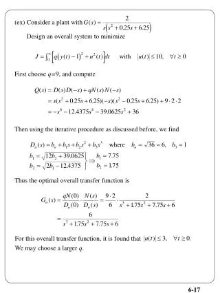
(ex) Consider a plant with. Design an overall system to minimize. First choose q= 9, and compute. Then using the iterative procedure as discussed before, we find. Thus the optimal overall transfer function is. For this overall transfer function, it is found that We may choose a larger q.

6-17
E N D
Presentation Transcript
(ex) Consider a plant with Design an overall system to minimize First choose q=9, and compute Then using the iterative procedure as discussed before, we find Thus the optimal overall transfer function is For this overall transfer function, it is found that We may choose a larger q. 6-17
6.5 ITAE Optimal Systems We discuss the design of control systems to minimize the integral of time multiplied by absolute error (ITAE). For the quadratic system the ITAE, IAE and ISE as a function of are shown below. The ITAE has largest changes as varies, and therefore has the best selectivity. The ITAE also yields a system with a faster response. The system that has the smallest ITAE is called the optimal system in the sense of ITAE. Consider the overall transfer function Because Go(s) is stable, the position error is zero. A table of system transfer functions has been prepared by Graham and Lathrop. They show the optimum form of the denominator, for systems whose transfer functions are of the form given by , which will minimize the ITAE. 6-18
Their poles and unit step responses for wo=1 are shown in the following figures. <Optimal pole locations> <Step responses of ITAE optimal systems with zero position error> 6-19
Let’s discuss the optimization of with respect to the ITAE criterion. By analog computer simulation, the optimal step responses of Go(s) are shown in the figure. <Step responses of ITAE optimal systems with zero velocity error> The optimal denominator of Go(s) are listed in the table. The systems are called the ITAE zero velocity error optimal systems. 6-20
Similarly, for the following overall transfer function the optimal step responses are shown in the figure and the optimal denominators are listed in the table. They are called the ITAE zero acceleration error optimal systems. Note that the optimal step responses for Go(s) in the previous figures are quite different. It seems that if a system is required to track a more complicated reference input, then the transient performance is poor. In other words, a price is paid if we design a more complex system. 6-21
- Application We discuss how to design ITAE optimal systems. (ex) Consider a plant with Find a zero position error system to minimize ITAE with The ITAE optimal overall transfer function is chosen as It is implementable. Also the larger , the faster the response. However, the actuating signal will also be larger. We need to choose to meet The transfer function from r to u is Then The largest u(t) can be computed by using the initial value theorem as Then we need to set Thus the ITAE optimal system is (ex) Consider the previous example with the additional requirement that the velocity error be zero. A possible is 6-22
However this is not implementable because of the pole-zero excess inequality. Now we choose the transfer function of degree 3. This is implementable and has zero velocity error. Now we need to choose so that The transfer function from r to u is Its unit step response is shown in the following figure. Note that the largest magnitude of u(t) does not occur at By computer simulation, we find that if Thus 6-23
6.6 Selection Based on Engineering Judgement We introduced two criteria : (1) minimization of the quadratic performance index, (2) minimization of ITAE. However in this section, we forgo the concept of minimization and select overall transfer functions based on engineering judgement. We require the system to have a zero position error and a good transient performance, i.e., small rise time, settling time, small overshoot. (ex) Consider plant with We use computer simulation to select two overall transfer functions The actuating signals of both systems due to a unit step input meet the constraint Then step responses are plotted in the following figure. 6-24
The step response of lies between those of the quadratic optimal system and the ITAE optimal system. Therefore is a viable alternative of the quadratic or ITAE optimal system. Consider It has a pair of complex conjugate poles as and a real pole of -10. The response of essentially dominated by the complex conjugate poles. However since the product of the three poles must equal 20, if we choose nondominant pole far away from the imaginary part, then the complex poles can’t be too far away from the origin of the s-plane. Thus its step response is slow. (ex) Consider a plant with We have designed a quadratic optimal system, i.e., and we have the ITAE optimal transfer function, i.e., or Now using computer simulation, we find the following has the response shown with the dashed-and-dotted line in the figure. We note that its response is comparable with that of the ITAE optimal system. 6-25
We have shown by examples that it is possible to use computer simulation to select an overall transfer function whose performance is comparable to that of the quadratic or ITAE optimal systems. In the search, we vary the coefficients of the quadratic or ITAE system and see whether the performance could be improved. If we do not have the quadratic or ITAE optimal systems as a starting point, it would be difficult to find a good system. 6.7 Summary Given is implementable if (1) there exists a configuration with no plant leakage such that can be built using only proper compensators (2) the resulting system is well-posed and totally stable. Then is implementable iff (1) is stable, (2) contains the nonminimum zeros of G(s), and (3) the pole zero excess of the pole zero excess of G(s). We discuss how to choose an implementable overall system to minimize the quadratic and ITAE performance indices. (i) quadratic optimal system After finding a spectral factorization, the optimal system can be obtained from (ii) ITAE optimal system ITAE Optimal system can be obtained from Tables. However, the tables are not exhaustive, for some plant transfer functions, no standard forms are available, thus we may resort to computer simulation. After obtaining quadratic, ITAE optimal systems, we may change the parameters of the optimal systems to see whether a move desirable system can be obtained. In conclusion, we should make full use of computers to carry out the design. 6-26