Download

1 / 23
230 likes | 249 Views
This article provides a concise recap of significance testing and explores the theory of significance testing. It also discusses the trial analogy and the concept of null and alternative hypotheses. The use of test statistics and p-values is explained, along with the necessary steps for inference using a confusion matrix. The significance test for the mean (T-Test) and other types of tests are introduced. Random comments and considerations for conducting significance tests in R are also provided.

E N D
Analysis of RT distributionswith R Emil Ratko-Dehnert WS 2010/ 2011 Session 06 – 14.12.2010
Before we start with R... • A concise recap of significance testing, as we will be computing tests with R today.
Excursion Theory of Significance Testing
Trial analgoy (I) • A Defendant is charged with a crime • Prosecutor and defense lawyer respectively must try to convice a jury of his guilt or innocence • Jurors are instructed to assume that the defendant is innocent, unless proven guilty beyond the shadow of a doubt
Trial analogy (II) • At the end jury decide guilt or innocence based on strength of their belief in the assumption of his innocence given the evidence • But: Convictions can be erroneous(!) • This depends on the threshold αused P( evidence | innocent) <=α
In our case... • H0 null hypothesis (formerly „innocent“) • H1 alternative (or research) hypothesis (formerly „guilty“) • One seeks to determine whether the H0is reasonable given the availible data (formerly „evidence“)
Test statistic and p-value • a test statistic is produced by an experiment and estimates the likelihood of data to H0 • p-value := P( test statistic is observed value or more | H0) • If p-value small -> test is statistically signifi-cant and casts doubt on H0
Inference: necessary steps • Identify H0, H1 • Specify a test statistic that discriminates between H0, H1; collect data and compute the test statistic • Using H1, specify values that are extreme under H0 in the direction of H1. • Calculate the p-value under H0. The smaller the value, the stronger the evidence against H0
Ex: calibration of a machine • A machine produces a „thingy“, with a specific height X ( X ~ N(0, 1); null hypothesis) • The height of a randomly chosen „thingy“ is 0.7 • Is the machine still in its tolerance band or has it slipped (e.g. X ~ N(1, 1); alternative hypothesis)?
area = 0.2420 area = 0.7580
area = 0.3821 area = 0.2420
Student‘s t-test (I) • Let the data X1, X2, ... Xn be an iid sequence, Xi~ N(μ, σ) (or n large enough for CLT) • A test of significance for can be performed with test statistic
Student‘s t-test (II) • T has the t-distribution with n-1 dof under H0 • Let t be an observed value of the test statistic, then the p-value is computed by
Other types • Test for the median • Test of proportion • Two sample test; Matched samples • Test over the rank (Wilcoxon) • ...
Random comments • Always check the assumption of the t-test (normality, independance, ...) • Statistical significance doesn‘t mean practical significance (look at effect size) • Repeated t-testing („testing into compliance“) has to be corrected to prevent α-inflation
Student‘s t-test in R • In R this is performed by the function t.test() t.test(x, mu= ..., alt = “two.sided“) • The output looks something like this
Quantile-quantile Plots • A q-q-plot plots the quantiles of one distribution against the quantiles of another as points. • If the distributions have similar shapes, the points will fall roughly along a straight line.
Quantile-quantile Plots • In R you can use the qqplot() function to check the distribution of two data set against each other • To check normality, one can use qqnorm() and add a reference line by qqline()