Download

1 / 41

E N D
ECN 2100 – INTERMEDIATE MICROECONOMICS Lecture 1 MATH REVIEW TOSHIA MC DONALD (JAMES), M.Sc. Department of Economics Faculty of Social Sciences, University of Guyana
Math Review & Working Tools Structure: • • • • Lecture session Questions for Discussion Activity Reading requirements
Why Math? • Mathematics is a very precise language, thus it is useful to express the relationships between related variables. Economics is the study of the relationships between resources and the alternative outputs hence math is a useful tool to express economic relationships. • Principles of Microeconomics Slide 3
Why Math? • In order to make Economic Analysis predictions, it is important to understand the basics of mathematics. For example we know that a decrease in supply will lead to an increase in demand. This is common sense when looking at rational consumer behaviours. In this scenario, the job of economists is to use mathematics to make proper precise predictions on how much demand will rise by. Principles of Microeconomics Slide 4
Relationships • A relationship between two or more variables can be expressed as an equation, table or graph – equations & graphs are “continuous” – tables contain “discrete” information • tables are less complete than equations • it is more difficult to see patterns in tabular data than it is with a graph -- economists prefer equations and graphs For Intermediate Microeconomics we will be using equations and graphs.
Equations • ……relationship between two variables can be expressed as an equation. the value of the “dependent variable” is determined by the equation and the value of the “independent variable.” the value of the independent variable is determined outside the equation, i.e. it is “exogenous” • • Principles of Microeconomics Slide 6
Equations • An equation asks when a function is equal to a particular number. • The solution to an equation is just a value of the variable or (variables) that makes the equation true. – y = 2x is a function – 3x = 9 is an equation • Answer: – x = 3 7
Functions and Graphs • Functions describe the (unique) relationship between two variables. – y = f(x) can be read as “y is a function of x” • We refer to y as the dependent variable and x as the independent variable because the value of y depends on the value of x. • Y = fi (X) says the value of Y is determined by the value of X A linear relationship may be specified: Y = a ± mX [the function will graph as a straight line] • When X = 0, then Y is “a” • for every 1 unit change in X, Y changes by “± m” 8
Functions and Graphs [Cont. . .] • E.g. Suppose y = f(x), where f(x) = 2x + 4 This means that The relationship between Y and X is determined; for each value of X there is one and only one value of Y [function] Substitute a value of X into the equation to determine the value of Y Values of X and Y may be positive or negative, for many uses in economics the values are positive – if x is 1, y must be 2(1) + 4 = 6 – if x is 2, y must be 2(2) + 4 = 8 • • • This relationship can also be described graphically. Principles of Microeconomics Slide 9
Graphing Functions y = 2x + 4 10 8 6 4 y 2 0 -2 -3 -2 -1 0 1 2 3 10 x
Graphing Functions Cont. A when X = 0 then Y = 6 [this is Y-intercept] A line that slopes from upper left to lower right represents an inverse or negative relationship, when the value of X increases, Y decreases! Y 6 sets of (X, Y) (0, 6) (1, 4) (2, 2) (3, 0) 5 when X = 1 then Y = 4 Given the relationship, Y = 6 - 2X, 4 3 When X = 2, then Y = 2 2 The relationship for all positive values of X and Y can be illustrated by the line AB 1 When X = 3, Y = 0, [this is X-intercept] B X 1 2 3 4 5 6 Principles of Microeconomics Slide 11
Graphing Functions Cont. Y Given a relationship, Y = 6 - .5X 6 (0,6) 5 (1,5.5) (2, 5) (4,4) (6,3) 4 For every one unit increase in the value of X, Y decreases by one half unit. The slope of this function is -.5! The Y-intercept is 6. 3 2 = 6 5 . = 0 , 12 , Y when X 1 What is the X-intercept? = 12 X 1 2 3 4 5 6
Properties of Functions • A function is called continuous - A function is said to be continuous in an interval if it is possible to draw the curve without any breakage. A function is continuous if all the points in the interval satisfy the function • A function is called smooth if it has no corners when drawn. • A function is monotonic if the dependent variable always increases or always decreases as the independent variable increases. 13
Linear Function – The Demand Function • Linear demand function – a relationship between quantity demanded and the market price q ap b = − + D – The relationship is negative since consumers buy less when the price gets higher
Demand and Supply Slope: price sensitivity Intercept: should be positive because consumers will buy something when the price is zero→satiation level
Inverse of a function • A function y = f(x) implies that for any value of x, there is a unique value of y. • The inverse of a function exists if there is also a unique value of x associated with each value of y. 16
Inverse Demand and Supply Functions • Economists prefer to put the price on the vertical axis – Historical tradition – The intercept of the supply function now has economic meaning, whether positive or negative • Inverse demand function is the demand function where the price is the dependent variable – More quantity in the market (less scarcity) makes prices fall • Inverse supply function is the supply function where the price is the dependent variable – Economic interpretation is more difficult
Identities • An identity is a relationship between variables that holds no matter what value is assigned to the variable. – (2x + y)2= 4x2+ 4xy + y2 – 6(x+2) = 6x + 12 20
Rate-of-Change and Slope • We are often interested in precisely how the dependent variable depends on the independent variable. – We want to know the rate-of-change of one variable relative to the other. • For example, how does the amount of output (y) change as a firm increases the quantity of an input (x)? • This is captured by the slope of a graph. 21
Rate-of-Change and Slope • For linear functions, this rate of change is constant and written as Δy/Δx. What is the linear function graphed below? y y 2 6 Rise Run -4 1 -2 4 2 2 2 4 x 3 4 x slope = Δy/Δx slope = Δy/Δx = -2/1 = -2 =(change in y)/(change in x) = -4/2 = -2 22
Slope of the Line • Negative Slope means that as one variable increases in value, the other one decreases, and vice versa. • Positive Slope means that as one variable increases in value so does the other, and vice versa. y y x x 23
Slope of the Line Cont’d Y 6 Y = 6 -.5X 5 as the value of X increases from 2 to 4, 4 D DY= -1 3 2 the value of Y decreases from 5 to 4 1 D DX = 2 X 1 2 3 4 5 6 D DY is the rise [or change in Y caused by D DX]{in this case, -1} so, slope is -1/2 or -.5 D DX is the run {+2}, rise run slope is
Slope of the Line Cont’d Y For a relationship, Y = 1 + 2X When X=0, Y=1 (0,1) When X = 1, Y = 3 slope = +2 6 5 (1,3) (2,5) When X = 2, Y = 5 4 rise +2 This function illustrates a positive relationship between X and Y. For every one unit increase in X, Y increases by 2 ! for a relationship Y = -1 + .5X slope = + 3 This function shows that for a 1 unit increase in X, Y increases 1 2 run +1 one half unit 2 rise +1 1 run +2 X 1 2 3 4 5 6 -1
Non-linear Functions • What happens when functions are “non-linear”? – Consider the functional relationship y = f(x), where f(x) = 3x2+ 1 y y slope = 24/2 = 12 slope = 9/1 = 9 28 24 13 9 4 4 2 1 1 3 1 2 x x • For non-linear relationships, Δy/Δx is a discrete approximation of the slope at any given point. – This approximation is better, the smaller the change in x we consider. 26
Non-linear Functions • We can also approximate the slope analytically: – Consider again the relationship y = f(x), where f(x) = 3x2+ 1 • Starting at x = 1, if we increase x by 2 what will be the corresponding change in y? f(1+2)- f(1) 2 =(3(3)2+1)-(3(1)2+1) =28-4 =12 2 2 • Similarly, starting at x = 1, if we increase x by 1 what will be the corresponding change in y? ) 1 + − ) 1 + ) 1 ( 3 ( − ) 1 + − 2 2 1 ( ) 1 ( ) 2 ( 3 ( 13 4 f f = = = 9 1 1 1 • So this functional relationship between x and y means that the change in y that results from a change in x depends on how big of a change in x and where you evaluate this ratio. 27
Computing the Rate of Change • Given a relationship between x and y such that y = f(x) for some function f(x), we have been considering the question of “if x increases by Δx, what will be the relative change in y?”, or x f x D D + D − ( ) ( ) y x f x = D x • For linear functions, the rate-of-change will always be constant. For example, if y = a + bx: • For non-linear functions, the rate of change depends on the value of x. For example, if y = x2 28
Derivative • When we have a nonlinear function, a simple derivative can be used to calculate the slope of the tangent to the function at any value of the independent variable ( the slope of a function at any given point) The notation for a derivative is written: • dY dX is the change in Y caused byachangein X " " Principles of Microeconomics Slide 29
The Derivative – Recall that we get a better approximation to the relative rate-of-change the smaller the change in x we consider. – The derivative is just the limit of this expression as Δx goes to zero, or f x + D − ( ) ( ) ( ) f x x x f x = lim D → 0 x D x • So going back to the example on the last slide as Δx goes to 0, the derivative is just 2x. – We will also sometimes express the derivative of f(x) as f’(x) 30
The Derivative • Given y = f(x), where f(x) = 3x2+ 1, what is the expression for the derivative? y So what is slope of f(x) = 3x2+ 1 at x = 1? 28 slope = ? – slope = ? 4 What is slope of f(x) = 3x2+ 1 at x = 3? – 1 3 x – How do we interpret these slopes? 31
Second Derivatives • The derivative of the derivative. • Intuitively, if the first derivative gives you the slope of a function at a given point, the second derivative gives you the slope of the slope of a function at a given point. – In other words, the second derivative is the rate-of-change of the slope. » If y = x2 dy dx=2x d2y dx2=d æ è ö ø dy dx ÷ =d dx2x =2 ç dx 32
Finding maxima and minima • Often calculus methods are used for finding what value maximizes or minimizes a function. – A necessary condition for an “interior” maximum or minimum is where the first derivative equals zero. y y f(x) f(x) x* x x* x 33
Local minima and maxima 10 8 x - 2 * sin(x) 6 4 2 0 0 2 4 6 8 10 34 x
Finding maxima and minima • This means that when trying to find where a function reaches its maximum or minimum, we will often take the first derivative and set it equal to zero – “ “First Order Condition” ” – f(x) = 10x – x2 – F.O.C.: 10 – 2x = 0 x* = 5 – How do we know if this is a maximum or a minimum? • f(x) has a minimum at x = a if f’(a) = 0 and f’’(a) > 0 • f(x) has a maximum at x = a if f’(a) = 0 and f’’(a) < 0 35
Partial Derivatives • Often we will want to consider functions of more than one variable. – For example: y = f(x, z), where f(x, z) = 5x2z + 2z – We will often want to consider how the value of such function changes when only one of its arguments changes. – This is called a Partial derivative 36
Partial Derivatives • The Partial derivative of f(x, z) with respect to x, is simply the derivative of f(x, z) taken with respect to x, treating z as just a constant. – Examples: • What is the partial derivative of f(x, z) = 5x2z3+ 2z with respect to x? – 10xz3 • With respect to z? 37
What Is Intermediate Microeconomics? • Intermediate Microeconomics is concerned with building models of economic behavior. – Two principles: • The Optimization Principle • The Equilibrium Principle • Our next topic is Consumer Choice: – How do economists model an individual’s choices? – What kinds of behavior is consistent/inconsistent? – Can we aggregate individual behavior into a discussion of consumer behavior more generally? 38
Questions • Open 39
EXERCISE • Graph the equation: Y = 9 - 3X – What is the Y intercept? The slope? – What is the X intercept? Is this a positive (direct) relationship or negative (inverse)? Graph the equation Y = -5 + 2X – What is the Y intercept? The slope? – What is the X intercept? Is this a positive (direct) relationship or negative (inverse)? • Principles of Microeconomics Slide 40
References • Math Review, https://slideplayer.com/slide/7584856/ • Chiang, Alpha C., Wainwright, Kevin, (2005), Fundamental Methods of Mathematical Economics. 4th (Forth) Edition, Mc Graw Hill-Irwin