A Look at More Complex Component-Based Applications
350 likes | 506 Views
A Look at More Complex Component-Based Applications. Component model for high performance computing. Components C++ objects with a functionality Ports : Provides and uses Compiled into shared libraries Framework Loads and instantiates components Connects uses and provides ports

A Look at More Complex Component-Based Applications
E N D
Presentation Transcript
Compaq Component model for high performance computing • Components • C++ objects with a functionality • Ports : Provides and uses • Compiled into shared libraries • Framework • Loads and instantiates components • Connects uses and provides ports • Driven by a script or GUI
Compaq A CCA code
Compaq CCA model for high performance computing • Requirements • High single cpu performance • Need parallelism, NOT distributed computing • SPMD quite sufficient, RMI not needed. • No parallel computing prescription/model • No one-size-fits-all • Translates to : • Light-weight framework • Onus on the component writer.
Compaq Component model for high performance computing • Solution : • Identical frameworks with identical components and connection on P processors. • Comp. A on proc Q can call methods on Comp. B also on proc Q. • Comp. A s of all P procs communicate via MPI. • No RMI – Comp. A on proc Q DOES NOT interact with Comp. B on proc N. • No parallel comp. Model – the component does what’s right. • 2 such frameworks – Sandia, Utah.
Compaq Pictorial example
Compaq Summary • A lightweight component model for high performance computing. • A restriction on parallel communication • Comm. Only between a cohort of components. • No RMI – no dist. computing. • Components with a physics / chemistry / numerical algo functionalities. • Standardized interfaces – Ports. • That’s the theory – does it work ?
Compaq Problem categories • Decomposition of simulation codes • How ? Along physics ? Numerics ? • Math model provides a hint ? • What granularity ? • Interfaces • Libraries • Interfaces • Nested containers • I.e. framework enhancements ?
Compaq Decomposition of simulation codes • 2 different physics simulations • Component reuse • Parallel, scalable, good single CPU performance • A formalism for decomposing a big code into • Subsystem • Components. • Common underlying mathematical structure • Dirty secrets / restrictions / flexibility.
Compaq Guidelines regarding apps • Hydrodynamics • P.D.E • Spatial derivatives • Finite differences, finite volumes • Timescales • Length scales
Compaq Solution strategy • Timescales • Explicit integration of slow ones • Implicit integration of fast ones • Strang-splitting
Compaq Solution strategy (cont’d) • Wide spectrum of length scales • Adaptive mesh refinement • Structured axis-aligned patches • GrACE. • Start with a uniform coarse mesh • Identify regions needing refinement, collate into rectangular patches • Impose finer mesh in patches • Recurse; mesh hierarchy.
Compaq A mesh hierarchy
Compaq App 1. A reaction-diffusion system. • A coarse approx. to a flame. • H2-Air mixture; ignition via 3 hot-spots • 9-species, 19 reactions, stiff chemistry • 1cm X 1cm domain, 100x100 coarse mesh, finest mesh = 12.5 micron. • Timescales : O(10ns) to O(10 microseconds)
Compaq App. 1 - the code
Compaq So, how much is new code ? • The mesh – GrACE • Stiff-integrator – CVODE, LLNL • ChemicalRates – old Sandia F77 subroutines • Diff. Coeffs – based on DRFM – old Sandia F77 library • The rest • We coded – me and the gang.
Compaq Evolution
Compaq Details • H2O2 mass fraction profiles.
Compaq App. 2 shock-hydrodynamics • Shock hydrodynamics • Finite volume method (Godunov)
Compaq Interesting features • Shock & interface are sharp discontinuities • Need refinement • Shock deposits vorticity – a governing quantity for turbulence, mixing, … • Insufficient refinement – under predict vorticity, slower mixing/turbulence.
Compaq App 2. The code
Compaq Evolution
Compaq Convergence
Compaq Are components slow ? • C++ compilers << Fortran compilers • Virtual pointer lookup overhead when accessing a derived class via a pointer to base class • Y’ = F ; [ I - t/2 J ] Y = H(Yn) + G(Ym) ; used Cvode to solve this system • J & G evaluation requires a call to a component (Chemistry mockup) • t changed to make convergence harder – more J & G evaluation • Results compared to plain C and cvode library
Compaq Components versus library
Compaq Really so ? • Difference in calling overhead • Test : • F77 versus componens • 500 MHz Pentium III • Linux 2.4.18 • Gcc 2.95.4-15
Compaq Scalability • Shock-hydro code • No refinement • 200 x 200 & 350 x 350 meshes • Cplant cluster • 400 MHz EV5 Alphas • 1 Gb/s Myrinet • Worst perf : 73 % scaling eff. For 200x200 on 48 procs
Compaq Summary • Components, code • Very different physics/numerics by replacing physics components • Single cpu performance not harmed by componentization • Scalability – no effect • Flexible, parallel, etc. etc. … • Success story …? • Not so fast …
Compaq Pros and cons • Cons : • A set of components solve a PDE subject to a particularnumerical scheme • Numerics decides the main subsystems of the component assembly • Variation on the main theme is easy • Too large a change and you have to recreate a big percentage of components • Pros : • Physics components appear at the bottom of the hierarchy • Changing physics models is easy. • Note : Adding new physics, if requiring a brand-new numerical algorithm is NOT trivial. • So what’s a better design to accommodate this ?
Compaq What else is up ? • “libraries” ! • But as components, standard interfaces • “Linear solver component” (interface!) • PetSc, Trilinos etc, etc • Meshes : • Standard interfaces for discretizing domains (unstructured meshes) • Math operators on such meshes • Data objects to hold fields on such meshes • Strange things … • Data de- and re-composition, visualization …
Compaq Libraries …. • Linear algebra • PETSc, Trilinos, etc components • Optimization • TAO • ODE & DAE Integrators • LSODE, Cvode • Profiling & optimization (cache artists ?!?) • TAU • Data redist + Viz • CUMULVS, using AVS, no less !
Black boxes: components • Blue boxes: provides ports • Gold boxes: uses ports Compaq Time-Dependent PDE on an Unstructured Mesh TSTT unstructured mesh prototype components with finite element discretizations. IntegratorLSODE provides a second-order implicit time integrator, and FEMDiscretization provides a discretization. This application uses the DADFactory component to describe the parallel data layout so that the CumulsMxN data redistribution component can then collate the data from a multi-processor run to a single processor for runtime visualization.
Compaq Heat Equation on an Adaptive Structured Mesh Solution of a two-dimensional heat equation on a square domain using a structured method. IntegratorLSODE provides a second-order implicit time integrator, and Model provides a discretization. The remaining components are essentially utilities that construct the global ODE system or adaptors that convert the patch-based data structures of the mesh to the globally distributed array structure used for runtime visualization.
Compaq Unconstrained Minimization Using a Structured Mesh Determine minimal surface area given boundary conditions using the TAOSolver optimization component. I.e., solve min f(x), where f: R R. n TAOSolver uses linear solver components that incorporate abstract interfaces under development by the DOE-wide Equation Solver Interface (ESI) working group. Underlying implementations are provided via the new ESI interfaces to parallel linear solvers within the PETSc (ANL) and Trilinos (SNL) libraries.
Compaq Conclusions • Progress .. • Libraries <-> components : well ahead • Decomposing applications • Slower, but harder job • Language interoperability • Framework done • Adoption by people on • Knotty points • Interfaces and scientists …