Seismic Interpretation and Subsurface Mapping
Seismic Interpretation and Subsurface Mapping. An A level teaching resource based on the Eakring oil field, East Midlands, UK Developed by Dorothy Satterfield (University of Derby) and Martin Whiteley (Barrisdale Ltd) on behalf of the Earth Science Teachers’ Association (ESTA) .


Seismic Interpretation and Subsurface Mapping
E N D
Presentation Transcript
Seismic Interpretation and Subsurface Mapping An A level teaching resource based on the Eakring oil field, East Midlands, UK Developed by Dorothy Satterfield (University of Derby) and Martin Whiteley (Barrisdale Ltd) on behalf of the Earth Science Teachers’ Association (ESTA)
Seismic Interpretation and Subsurface Mapping • Introduction • Basic principles • Eakring exercise • Additional information
1. Introduction • Seismic interpretation and subsurface mapping are key skills that are used commonly in the oil industry • This teaching resource introduces the basic principles of seismic interpretation and then, if time permits, they can be applied in a practical exercise • The resource dovetails with the A level Geology specifications
2. Basic principles • Seismic acquisition • Seismic processing • Understanding the data • Seismic interpretation
Seismic acquisition offshore • An air gun towed behind the survey ship transmits sound waves through the water column and into the subsurface • Changes in rock type or fluid content reflect the sound waves towards the surface • Receivers towed behind the vessel record how long it takes for the sound waves to return to the surface • Sound waves reflected by different boundaries arrive at different times. • The same principles apply to onshore acquisition
Seismic acquisition onshore (1) • Onshore seismic acquisition requires an energy input from a “thumper” truck. Geophones arrayed in a line behind the truck record the returning seismic signal. Vibrator (source) Geophones (receivers) Sub-horizontal beds Unconformity Dipping beds
Seismic horizons represent changes in density and allow the subsurface geology to be interpreted. Seismic acquisition onshore (2) Lithology change Angular unconformity Lithology change
Seismic processing • Wiggle trace to CDP gather • Normal move out correction • Stacking • What is a reflector?
Wiggle trace to CDP gather Wiggle traces CDP gather Graphs of intensity of sound as received by the recorders Graphs of intensity for one location collected into groups and shown in a sequence.
1 2 Normal move out correction CMP Sound sources S1 S2 S3 Sound receiversR3 R2 R1 Slowest Fastest Wave reflected Sound wave in Change in lithology from mud to sand so sound is reflected back to surface CDP Data for one point from different signals to different receivers 1. More time needed to reach distant receivers so the data look like a curve. 2. Correcting for normal move out restores the curve to a near horizontal display. Original CDP gather … corrected for normal move out
First, gather sound data for one location and correct for delayed arrival (normal move out) Next, take all the sound traces for that one place and stack them on top of each other Finally, place stacks for adjacent locations side by side to produce a seismic line Stacking
energy source signal receiver Reflected ray Bed 1 Incoming ray lower velocity higher velocity Refracted ray Bed 2 What is a reflector? A seismic reflector is a boundary between beds with different properties. There may be a change of lithology or fluid fill from Bed 1 to Bed 2. These property changes cause some sound waves to be reflected towards the surface. There are many reflectors on a seismic section. Major changes in properties usually produce strong, continuous reflectors as shown by the arrow.
Understanding the data • Common Depth Points (CDPs) • Floating datum • Two way time (TWT) • Time versus depth
Common Depth Points Common midpoint above CDP Sound sources S1 S2 S3 Sound receiversR3 R2 R1 CDPs are defined as ‘the common reflecting point at depth on a reflector or the halfway point when a wave travels from a source to a reflector to a receiver’. Sound wavereflected Sound wave in Change in lithology = reflecting horizon Common reflecting point or common depth point (CDP)
The topographic elevation is the height above sea level of the surface along which the seismic data were acquired. Floating datum The floating datum line represents travel time between the recording surface and the zero line (generally sea level). This travel time depends on rock type, how weathered the rock is, and otherfactors.
Two way time (TWT) Two way time (TWT) indicates the time required for the seismic wave to travel from a source to some point below the surface and back up to a receiver. In this example the TWT is 0.5 seconds. TWT surface 0 0.25 seconds 0.25 seconds 0.5 seconds
288 0.58 sec 926 m 926 1865 m Time versus depth • Two way time (TWT) does not equate directly to depth • Depth of a specific reflector can be determined using boreholes • For example, 926 m depth = 0.58 sec. TWT
Seismic interpretation • Check line scale and orientation. • Work from the top of the section, where clarity is usually best, towards the bottom. • Distinguish the major reflectors and geometries of seismic sequences.
Scale and orientation • Use the scale bar to estimate the length of the line • Use CDPs to check theorientation of the line on the accompanying map
first second third • Start at the top of the section, where definition is usually best • Work down the section toward the zone where the signal to noise ratio is reduced and the reflector definition is less clear Top down approach
Reflector character and geometry Continuous reflector truncating short ones Next continuous reflector Reflectors onlapping continuous one
3. Eakring exercise This exercise has been developed to illustrate, in practice, how subsurface information can be integrated and used to predict where an oilfield may occur. It builds on the principles outlined in the PowerPoint presentation and can be completed by individuals or small teams according to the time available or their level of enthusiasm. The seismic lines and base map can be obtained from Dorothy Satterfield (d.satterfield@derby.ac.uk) in a format that is suitable for photocopying on A3 paper. You will also receive a CD that contains a copy of the entire PowerPoint presentation that you can customise as you wish. This is free! The aim is to interpret the seismic data and then produce a map that shows the subsurface structure in the region of the Eakring oil field. Oil fields typically form in simple dome-like structures in the subsurface. The structure must enclose porous and permeable rocks that are capable of containing oil and in this example there are a number of potential reservoirs developed in the Namurian and Westphalian (Carboniferous) sandstones. Oil is prevented from leaking to the surface by overlying mudstones and coals which are impermeable.
Background information Oil exploration in the East Midlands has a long history. Eakring and the neighbouring Dukes Wood oil fields were discovered in the 1930s. Most oil wells at Dukes Wood date from World War II, though this ‘nodding donkey’ or oil pump may be a little younger. Production at Eakring and Dukes Wood was important to the war effort in Britain. Oil production at Dukes Wood stopped in 1966, but it continued in Eakring until 2003.
Project data Map showing the location of the 5 seismic lines The seismic data were acquired in 1984 (hence the prefix “84” to each line number) Notice also the Eakring Village well and the location of oil fields in the area
Understanding the data (1) CDPs are typically marked at intervals along the top of seismic lines and they are regularly spaced to form a horizontal scale. Here, 80 CDPs represent about 1 kilometre (km).
Understanding the data (2) Gaps in land seismic data are due to omissions where data could not be acquired For example, it is not always possible to transmit the signal above pipes, in sensitive areas and above buildings Signals from farther away will provide information for deeper horizons
Understanding the data (3) Two way time (TWT) is recorded on the vertical axis of the seismic line in fractions of a second. Sometimes it is more convenient to express time as milliseconds. TWT is the time required for the seismic wave to travel from the source to some point below the surface and back up to the receiver. 0.0 seconds or sea level 0.5 seconds or 500 milliseconds 1.0 seconds or 1000 milliseconds
Correlating well and seismic data • Use the Eakring Village well, which is located near the intersection of lines 69 and 70, to tie seismic reflectors to known geological horizons identified in the well: • Base Permian at 150 milliseconds • Blackshale Coal at 240 milliseconds • Near Top Dinantian at 500 milliseconds • The potential reservoirs are Namurian and Westphalian (Upper Carboniferous) sandstones that occur below the Blackshale Coal and above the Near Top Dinantian (Lower Carboniferous) horizon
Well tie to seismic -0.2 -0.1 0.0 0.1 0.2 0.3 0.4 0.5 1.0 Eakring Village (projected) Eakring Village (projected) Base Permian 150 ms Base Permian 150 ms Potential reservoir interval Blackshale Coal 240 ms Blackshale Coal 240 ms Near Top Dinantian 500 ms Two Way Time (TWT) in Seconds
Correlating reflectors Starting at the top of the section, interpret the Base Permian unconformity away from the well on line 69 and correlate it with intersecting lines 70 and 71. Continue this process around the ‘loops’ formed by lines 72 and 73, ensuring that your interpretation is consistent and geologically reasonable. Repeat this process for the Blackshale Coal and Near Top Dinantian reflectors, accepting that in some areas the data quality is quite poor and a ‘best-guess’ interpretation is necessary. It may be helpful to annotate the lines to highlight where possible faults disrupt the gentle dip of the Blackshale Coal.
Correlating the Base Permian unconformity Eakring Village (projected) Start by interpreting the Base Permian unconformity away from the well on line 69. Next fold line 70 at the intersection with line 69 and match them up. Find and interpret the Base Permian unconformity. Finally, unfold line 70 and finish the interpretation.
Plotting the Base Permian data Determine the time values (in milliseconds) for the Base Permian at an appropriate CDP interval and plot those values on the map. For example, on line 69 you could start by plotting values at CDP 500, 600, 700, 800 and so on. 160 ms 150 ms 150 ms 150 ms Base Permian unconformity 150 ms 150 ms 160 ms 150 ms
Mapping the Blackshale Coal • Because the potential reservoir interval is poorly imaged (the reflectors are weak and discontinuous) the closest and most prominent reflector to map is the overlying Blackshale Coal. • Determine the time value (in milliseconds) for the Blackshale Coal at an appropriate CDP interval and plot that value on the map. For example, on line 69 you could start by plotting values at CDP 500, 600, 700, 800 and so on. In some areas it may be necessary to infill with data at a finer scale. • Contour these values to make a time map. Take particular care to recognise where faults may complicate the interpretation. • Normally, a time map is converted into a depth map using velocity functions, but for the purpose of this exercise the time/depth pairings at the top of each seismic line give an adequate representation of the depth to a given horizon.
Plotting data for the Blackshale Coal In some cases it may be easier to choose convenient time values for contouring (say, 250 ms, 300 ms, 350 ms, etc.) and plot these against the appropriate CDPs. 250 250 250 250 280 210
Contouring the data Use the time values to produce contours. Label them in milliseconds to create a subsurface time structure map. 300 250 250 250 300 210 250 300 300 250 250
Interpreting the map 1. What does the map show? 2. Using the time/depth pairings, what is the approximate depth in metres to the top of the potential reservoir interval at the crest of the mapped structure? To answer this, plot the time/depth pairings on a graph, insert a line of best fit and use it to derive the approximate depth of the reservoir interval. 3. Where would you locate additional seismic data to confirm the size and shape of the potential structural trap that you have mapped?
4. Additional information • Specimen ‘answers’ • Extension activities • Web-based resources • Further reading • Contact us • Acknowledgements
Specimen ‘answers’ The Blackshale Coal dips gently towards the NE and reaches a high point in the vicinity of the intersection of lines 69 and 70. Faults can be extrapolated in a variety of ways in the SW part of the map to create a potential trap. 1. The crest of the potential structure as defined by the Blackshale Coal is at 210 milliseconds (at CDP 540 on line 69), but the potential reservoir unit is at about 300 milliseconds. Inspection of the time/depth pairings in the area shows that 300 milliseconds corresponds to about 350 metres below surface. 2. The potential trap would need to be better defined by extending the seismic lines in a southerly direction. The extent of the Eakring Field is shown on the seismic line location map (Slide 24) and it is evidently an elongate N-S structure, of which only the northernmost culmination is defined in this exercise. 3.
Extension activities Individuals or groups with sufficient time and interest may want to tackle one of the following activities: • Research the economic and social impact of the wartime extraction of oil from the East Midlands • Analyse the similarities and differences between onshore and offshore oil exploration in the UK • Assess the remaining potential of onshore oil and gas in the UK • Account for the differences between the small oil fields in the East Midlands and the much larger accumulation at Wytch Farm in Dorset
Web-based resources (1) • This website, developed by the University of Tromsø in Norway, contains a number of modules that summarise key geological topics through simple animated cartoons. In particular, the ‘Oil and Gas’ module provides useful background information for teachers and students who may not be conversant with hydrocarbon geology. http://www.ig.uit.no/webgeology/
Web-based resources (2) • Oil and Gas UK provides educational information on its website including history of the North Sea and exploration and production techniques. http://www.oilandgas.org.uk/education/index.cfm • More specifically, Oil and Gas UK, with the support of the Natural History Museum, has produced online and paper versions of Britain's Offshore Oil and Gas , which isan excellent introduction to the history, science and technology of the UK oil industry. http://www.oilandgas.org.uk/education/storyofoil/index.cfm
Web-based resources (3) • The UK Onshore Geophysical Library manages the archive and official release of seismic data recorded over landward areas of the UK. One of the Library's main objectives is to provide active support for academia, and there is limited support for provision of data to educational institutions. http://www.ukogl.org.uk/
Web-based resources (4) • This report, produced by the British Geological Survey (BGS) on behalf of the Department of Trade and Industry (DTI), provides a general synopsis of the petroleum systems of the UK’s onshore basins • It is a large (6MB) file that may take some time to open and download http://www.og.dti.gov.uk/UKpromote/geoscientific/ Onshore_petroleum_potential_2006.pdf
Web-based resources (5) • This website provides information about the Dukes Wood Oil Museum and Nature Reserve, near Eakring. It is an interesting place to visit because it combines both natural and industrial history. School parties are welcome and the reserve is always open, but access to the oil museum needs to be pre-arranged http://www.dukeswoodoilmuseum.co.uk/
Further reading The Sedimentary Record of Sea-Level Change, edited by Angela L. Coe, 2003. Co-published by The Open University and Cambridge University Press, 288 pages. A regional assessment of the intra-Carboniferous play of Northern England, by Fraser, A. J. et al. in Classic Petroleum Provinces, edited by Jim Brooks, 1990. Geological Society Special Publication No. 50, pp.417-440.
Contact us Dr Dorothy Satterfield Geography, Earth, and Environmental Sciences University of Derby (FEHS) Kedleston Road Derby DE22 1GB Email: d.satterfield@derby.ac.uk Dr Martin J Whiteley Barrisdale Limited 16 Amberley Gardens Bedford MK40 3BT Email: mjwhiteley@yahoo.co.uk
Acknowledgements Data, images and advice were provided by the following individuals and organisations:Mark Alldred from the UK Onshore Geophysical Library (UKGOL) Oil and Gas UK for permission to reproduce data contained in Slides 5 and 9-11 Tony Hodge and Mick Price from Roc Oil