Download
1 / 39
390 likes | 738 Views
The Classical Long-Run Model. Economists sometimes disagree with each other Actually much more agreement exists among economists than there appears to be Once distinction between long-run and short-run becomes clear Many apparent disagreements among macroeconomists dissolve

E N D
The Classical Long-Run Model • Economists sometimes disagree with each other • Actually much more agreement exists among economists than there appears to be • Once distinction between long-run and short-run becomes clear • Many apparent disagreements among macroeconomists dissolve • If no time horizon is specified, however, an economist is likely to focus on horizon he or she feels is most important • Something about which economists sometimes do disagree
The Classical Long-Run Model • Ideally, we would like our economy to do well in both long-run and short-run • Unfortunately, there is often a trade-off between these two goals • Doing better in short-run can require some sacrifice of long-run goals, and vice versa • Policies that can help us smooth out economic fluctuations may prove harmful to growth in the long-run • While policies that promise a high rate of growth might require us to put up with more severe fluctuations in short-run
Macroeconomic Models: Classical Verses Keynesian • Classical model, developed by economists in 19th and early 20th centuries, was an attempt to explain a key observation about economy • Over periods of several years or longer, economy performs rather well • If we think in terms of decades rather than years or quarters, business cycle fades in significance • In the classical view, this behavior is no accident • Powerful forces are at work that drive economy towards full employment • An important group of macroeconomists continues to believe that classical model is useful even in shorter run • In 1936, in midst of Great Depression, British economist John Maynard Keynes offered an explanation for economy’s poor performance • Argued that, while classical model might explain economy’s operation in long-run, long-run could be a very long time in arriving
Macroeconomic Models: Classical Verses Keynesian • Keynesian ideas became increasingly popular in universities and government agencies during 1940s and 1950s • By mid-1960s, entire profession had been won over • Macroeconomics was Keynesian economics • Classical model was removed from virtually all introductory economics textbooks • Classical model is still important • In recent decades there has been an active counterrevolution against Keynes’s approach to understanding the macroeconomy • Useful in understanding economy over long-run • While Keynes’s ideas and their further development help us understand economic fluctuations—movements in output around its long-run trend • Classical model has proven more useful in explaining the long-run trend itself
Assumptions of the Classical Model • All models begin with assumptions about the world • Classical model is no exception • Many of its assumptions are simplifying • Make model more manageable, enabling us to see the broad outlines of economic behavior without getting lost in details • One assumption in classical view that goes beyond mere simplification-critical assumption • Markets clear • Price in every market will adjust until quantity supplied and quantity demanded are equal
Assumptions of the Classical Model • Market-clearing assumption provides hint about why classical model does a better job over longer time periods (several years or more) than shorter ones • We’ll use classical model to answer a variety of important questions about economy in long-run, such as • How is total employment determined? • How much output will we produce? • What role does total spending play in the economy? • What happens when things change?
How Much Output Will We Produce? • How can we disentangle web of economic interactions we see around us? • Decide which market or markets best suit the problem being analyzed, and • Identify buyers and sellers • Identify type of environment in which they trade • But which market should we start with? • Logical start is market for resources • Labor, land and natural resources, capital and entrepreneurship • We’ll concentrate our attention on labor • Our question is • How many workers will be employed in the economy?
Real Hourly Wage Excess Supply of Labor $20 15 Number of Workers Figure 1: The Labor Market LS B A E H J 10 Excess Demand for Labor LD 100 million = Full Employment
The Labor Market • Labor supply curve slopes upward • Because—as wage rate increases—more and more individuals are better off working than not working • Thus, a rise in wage rate increases number of people who want to work—to supply their labor • As wage rate increases each firm will find that—to maximize profit—it should employ fewer workers than before • When all firms behave this way together a rise in wage rate will decrease quantity of labor demanded • This is why economy’s labor demand curve slopes downward • In classical view, economy achieves full employment on its own
Determining the Economy’s Output • Most effective way to master a macroeconomic model is “divide and conquer” • Start with part of model, understand it well, and then add in other parts • Accordingly, our classical analysis of economy is divided into two separate questions • What would be the long-run equilibrium of the economy if there were a constant state of technology • And if quantities of all resources besides labor were fixed? • What happens to this long-run equilibrium when technology and quantities of other resources change?
The Production Function • Relationship between total employment and total production in the economy • Given by economy’s aggregate production function • Shows total output economy can produce with different quantities of labor • Given constant amounts of other resources and current state of technology • In classical, long-run view economy reaches its potential output automatically • An important conclusion of classical model and an important characteristic of the economy in long-run: • Output tends toward its potential, full-employment level on its own, with no need for government to steer the economy toward it
Real Hourly Wage In the labor market, the demand and supply curves intersect to determine employment of 100 million workers. Number of Workers Output (Dollars) The production function shows that those 100 million workers can produce $7 trillion of real GDP. Number of Workers Figure 2: Output Determination in the Classical Model LS $15 LD 100 million Aggregate Production Function $7 Trillion = Full Employment Output 100 million
The Role of Spending • What if business firms are unable to sell all output produced by a fully employed labor force? • Economy would not be able to sustain full employment for very long since business firms will not continue to employ workers who produce output that is not being sold • If we are asserting that potential output is an equilibrium for the economy • Had better be sure that total spending on output is equal to total production during the year • But can we be sure of this? • In classical view answer is yes
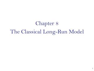
Total Spending in a Very Simple Economy • Imagine a world with just two types of economic units • Households and business firms • Circular Flow • A diagram that shows how goods, resources, and dollar payments flow between households and firms • In a simple economy with just households and firms in which households spend all of their income without saving it or paying tax • Total spending must be equal to total output • Known as Say’s Law
Households Goods Markets Factor Markets Firms Figure 3: The Circular Flow Goods and Services Demanded Resources Supplied $ Total Consumption Spending $ Total Income $ Total Revenue of Firms $ Total Factor Payments Goods and Services Supplied Resources Demanded
Total Spending in a Very Simple Economy • Say’s Law named after classical economist Jean Baptiste Say (1767-1832), who popularized the idea • Each time a god or service is produced, an equal amount of income is created, For example, each time a shirt manufacturer produces a $25 shirt, it creates $25 in factor payments to households. • In Say’s own words • “A product is no sooner created than it, from that instant, affords a market for other products to the full extent of its own value…Thus, the mere circumstance of the creation of one product immediately opens a vent for other products” • Say’s law states that by producing goods and services • Firms create a total demand for goods and services equal to what they have produced or more simply • ‘Supply creates its own demand’
Total Spending in a More Realistic Economy • Does Say’s law also apply in a more realistic economy? • In the real world • Households don’t spend all their income • Rather, some of their income is saved or goes to pay taxes • Households are not the only spenders in the economy • Businesses and government buy some of the final goods and services we produce • In addition to markets for goods and resources, there is also a loanable funds market • Where household saving is made available to borrowers in business or government sectors
Some New Macroeconomic Variables • Planned investment spending (IP) over a period of time is total investment spending (I) minus change in inventories over the period • IP = I – Δ inventories • Net taxes (T) are total government tax revenue minus government transfer payments (unemployment insurance, welfare payments, Social Security benefits) • T = total tax revenue – transfers • Household saving (S) • It’s often useful to arrive at household saving in two steps • Determine how much income household sector has left after payment of net taxes • Household sector’s disposable income • Disposable Income = Total Income – Net Taxes • Part that is not spent is defined as (household) saving (S) • S = Disposable Income – C
Some New Macroeconomic Variables • Total Spending in Classica • In Classica, total spending is sum of purchases made by household sector (C), business sector (IP), and government sector (G) • Total spending = C + IP + G • Saving and net taxes are called leakages out of spending • Amount of income that households receive, but do not spend • There are also injections—spending from sources other than households • A government’s purchases of goods and services • Planned investment spending (IP) • Total spending will equal total output if and only if total leakages in the economy are equal to total injections • Only if sum of saving and net taxes is equal to sum of planned investment spending and government purchases
G ($1.25 ($2 T Trillion) Trillion) G ($2 Trillion) IP ($1.75 ($1 S Trillion) Trillion) IP ($1 Trillion) $7 Trillion $7 Trillion C C ($4 Trillion) ($4 Trillion) Total Total Total Output Income Spending Figure 4: Leakages and Injections Leakages Injections =
The Loanable Funds Market • Where households make their saving available to those who need additional funds • Total supply of loanable funds is equal to household saving • Funds supplied are loaned out, and households receive interest payments on these funds (if the funds are provided through stock market then?) • Businesses’ demand for loanable funds is equal to their planned investment spending • Funds obtained are borrowed, and firms pay interest on their loans • Budget deficit • Excess of government purchases over net taxes • Budget surplus • Excess of net taxes over government purchases • When government purchases of goods and services (G) are greater than net taxes (T) • Government runs a budget deficit equal to G – T • When government purchases of goods and services (G) are less than net taxes (T) • Government runs a budget surplus equal to T - G
The Loanable Funds Market • When the government runs a budget deficit, its demand for loanable funds is equal to its deficit. The funds are borrowed, and government pays interest on its loans. • View of the loanable funds market: • The supply of funds is household saving • The demand for funds is the sum of the business sector’s planned investment spending and the government sector’s budget deficit, if any.
The Supply of Funds Curve • Since interest is reward for saving and supplying funds to financial market • Rise in interest rate increases quantity of funds supplied (household saving), while a drop in interest rate decreases it • Supply of funds curve • Indicates level of household saving at various interest rates • Quantity of funds supplied to the financial market depends positively on interest rate • This is why the saving, or supply of funds, curve slopes upward • Other things can affect savings besides the interest rate, including • Tax rates • Expectations about the future • General willingness of households to postpone consumption
As the interest rate rises, saving or the quantity of loanable funds supplied increases. Interest Rate Trillions of Dollars per Year Figure 5: Supply of Household Loanable Funds Saving (S) or Supply of Funds B 5% A 3% 1.5 1.75
The Demand for Funds Curve • When interest rate falls investment spending and the business borrowing needed to finance it rise • Business demand for funds curve slopes downward • What about government’s demand for funds? • Will it, too, be influenced by the interest rate? • Probably not very much • Government seems to be cushioned from cost-benefit considerations that haunt business decisions • Any company president who ignored interest rates in deciding how much to borrow would be quickly out of a job • U.S. presidents and legislators have often done so with little political cost • Government sector’s deficit and its demand for funds are independent of interest rate • As interest rate decreases quantity of funds demanded by business firms increases • While quantity demanded by government remains unchanged • Therefore, total quantity of funds demanded rises
As the interest rate falls, business firms demand more loanable funds for investment projects. Interest Rate Trillions of Dollars per Year Figure 6: Business Demand for Loanable Funds A 5% B 3% Planned Investment (IP) or Business Demand for Funds 1.0 1.5
. . . and the govern-ment's demand for loanable funds . . . Summing business demand for loanable funds at each interest rate . . . gives us the economy's total demand for loanable funds at each interest rate. Interest Rate Government Demand for Funds (G – T) Total Demand for Funds [IP + (G – T)] Business Demand for Funds (IP) B B B 5% A A A 3% 1.0 1.5 0.75 1.75 2.25 Trillions of Dollars per Year Trillions of Dollars per Year Trillions of Dollars per Year Figure 7: The Demand for Funds
Equilibrium in the Loanable Funds Market • In classical view loanable funds market is assumed to clear • Interest rate will rise or fall until quantities of funds supplied and demanded are equal • Can we be sure that all output produced at full employment will be purchased?
Interest Rate Trillions of Dollars Figure 8: Loanable Funds Market Equilibrium Total Supply of Funds (S) 5% E Total Demand for Funds [IP + (G – T)] 1.75
The Loanable Funds Market and Say’s Law • As long as loanable funds market clears, Say’s law holds • Total spending equals total output • This is true even in a more realistic economy with saving, taxes, investment and government deficit • Here’s another way to see the same result, in terms of a simple equation • Loanable funds market clears S = IP + (G – T) • Rearranging this equation by moving T to left side • Loanable funds market clears S + T = IP + G • Say’s law shows that total value of spending in economy will equal total value of output • Rules out a general overproduction or underproduction of goods in the economy • It does not promise us that each firm will be able to sell all of the particular good it produces
Loanable Funds Market Leakages Injections G ($2 Trillion) T ($1.25 Trillion) G ($2 Trillion) IP ($1 Trillion) S ($1.75 Trillion) IP ($1 Trillion) = $7 Trillion $7 Trillion C C ($4 Trillion) ($4 Trillion) Total Output Total Income Total Spending Figure 9: An Expanded Circular Flow $1.75 Trillion $1.0 Trillion $0.75 Trillion $1.25 Trillion
The Classical Model: A Summary • Began with a critical assumption • All markets clear • In classical model, government needn’t worry about employment • Economy will achieve full employment on its own • In classical model, government needn’t worry about total spending • Economy will generate just enough spending on its own to buy output that a fully employed labor force produces
Using the Theory: Fiscal Policy in the Classical Model • Could government increase economy’s total employment and total output by raising total spending? Seems like an idea that should work? ..business firms might hire more workers and produce more? • Two ideas for increasing spending come to mind • Government could simply purchase more output itself • More goods, like tanks and police cars, or more services, like those provided by high school teachers and judges • Government could cut net taxes, letting households keep more of their income • So they would spend more on food, clothing, furniture, new cars, and so on
Fiscal policy in the CM • Fiscal policy is a change in government purchases or in net taxes • Designed to change total spending in the economy and thereby influence levels of employment and output • Idea behind fiscal policy sounds sensible enough • But does it work? • Not if economy behaves according to classical model • Fiscal policy in classical model is completely ineffective. It can’t change total output or total employment • It can’t even change total spending • Moreover Fiscal policy is unnecessary (?) since the economy achieves and sustains full employment on its own
Using the Theory: Fiscal Policy With A Budget Deficit • What would happen if the government of Classica—which is running a deficit—attempted to increase employment and output by increasing government purchases • Crowding out is a decline in one sector’s spending caused by an increase in some other sector’s spending • In classical model a rise in government purchases completely crowds out private sector spending so total spending remains unchanged • In classical model, an increase in government purchases has no impact on total spending and no impact on total output or total employment • Opposite sequence of events would happen if government purchases decreased • Total spending and total output would remain unchanged
Interest Rate Funds ($ Trillions) Figure 10: Crowding Out With An Initial Budget Deficit Total Supply of Funds (S) 7% B D IP A C H 5% DC D2 D1 1.75 2.05 2.25
Fiscal Policy With A Budget Surplus • Total spending remains unchanged, and fiscal policy is completely ineffective • Same conclusion we reached about fiscal policy with a government budget deficit • Our exploration of fiscal policy shows us that, in long-run • Government efforts to change total output by changing government spending or taxes are unnecessary and ineffective
Funds ($ Trillions) Figure 11: Crowding Out With An Initial Budget Surplus S2 S1 B 7% DIP H C 5% A DC Business Demand for funds (IP) 1.25 1.55 1.75