Download
1 / 41
410 likes | 577 Views
RMI Workshop - Genetic Algorithms. Genetic Algorithms and Related Optimization Techniques: Introduction and Applications. Kelly D. Crawford ARCO Crawford Software, Inc. Other Optimization Colleagues. Donald J. MacAllister ARCO Michael D. McCormack Richard F. Stoisits

E N D
RMI Workshop - Genetic Algorithms Genetic Algorithms and Related Optimization Techniques: Introduction and Applications Kelly D. Crawford ARCO Crawford Software, Inc.
Other Optimization Colleagues Donald J. MacAllister ARCO Michael D. McCormack Richard F. Stoisits Optimization Associates, Inc.
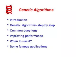
A “no hype” introduction to genetic algorithms (GA) What every “intro to GAs” talk begins with: - Biology - Evolution - Survival of the fittest What I am not going to talk about: - Biology - Evolution - Survival of the fittest - Exception: nomenclature/jargon It’s not about biology - it’s about search!
Optimization Given a potential solution vector to some problem: x Any set of constraints on x: Ax b And a means to assess the relative worth of that solution: f(x) (which may be continuous or discrete) Optimization describes the application of a set of proven techniques that can find the optimal or near optimal solution to the problem. Examples of optimization techniques: Genetic algorithms, genetic programming, simulated annealing, evolutionary programming, evolution strategies, classifier systems, linear programming, nonlinear programming, integer programming, pareto methods, discrete hill climbers, gradient techniques, random search, brute force (exhaustive search), backtracking, branch and bound, greedy techniques, etc...
Optimization Application Examples at ARCO Gas lift optimization (Ashtart): x: Amount of gas injected into each well Ax b: Max total gas available, max water produced f(x): Total oil produced Technique: Learning bit climber Free Surface Multiple Suppression: x: Inverse source wavelet Ax b: Min/max wavelet amplitudes f(x): Total seismic energy after wavelet is applied Technique: Genetic algorithm and learning bit climber
What to look for in an Optimization Technique Convergent techniques: continuous: Gradient search, linear programming discrete: Integer programming, gradient estimators Ok for search spaces with asingle peak/trough Divergent techniques: Random search, brute force (exhaustive search) Ok for small search spaces Hard problems (large search spaces, multiple peaks/troughs) need both convergent and divergent behaviors Genetic algorithms, simulated annealing, learning hill climbers, etc. These techniques can exploit the peaks/troughs, as well as intelligently explore the search space.
Convergent and Divergent Behaviors Need a balanced combination of both convergent ( ) and divergent ( ) behaviors to find solutions in complicated search spaces.
Genetic Algorithms - A Sample Problem • Ashtart gaslift optimization • 24 wells - Offshore Tunisia • Given: A fixed amount of gas for injection • Question: What is the right amount of gas to inject into each well to maximize oil production?
Gathering Lines Facility Lift Gas Production Well Lift Gas Optimization Lift Gas Curve • Objective • Maximize oil production rate. • No capital expenditures. Total Oil Produced Total lift gas
.882736363 1001010011010……0000101001111010011110……10011100101100 1100101100 1001010011 0100111101 .587467362 .287328726 Genetic Algorithms - Representing a Solution Chromosome Genotype Genes ... ... ... ... Phenotype Well 1 Well 12 Well 24
10 01010011 00 11011010 0001010011 0001011011 Genetic Algorithms - Crossover and Mutation • Genetic Operations on Chromosomes - Crossover Parents Children 00 01010011 10 11011010 • Genetic Operations on Chromosomes - Mutation
x = 1001010011010……0000101001111010011110……10011100101100 f(x) ==> 19020.234789 Genetic Algorithms - Evaluating a Solution’s Fitness So just how good are you, kid…? Total Daily Oil Production for the Field
1001010011 0001110001 0101100010 1101110010 Y B X A 1000011101 1011011111 Z 0001110111 0000000101 1111010000 0101010010 Done? Genetic Algorithms - The Process Parents Children A B Crossover and Mutation X Y Z No Yes
What are the necessary requirements for using a GA? When you need… ...some way to represent potential solutions to a problem (representation: bit string, list of integers or floats, permutation, combinations, etc). ...some way to evaluate a potential solution resulting in a scalar. This will be used by the GA to rank the worth of a solution. This fitness (or evaluation) function needs to be very efficient, as it may need to be called thousands - even millions - of times. But you do not need... ...the final solution to be optimal. ...speed (this varies)
When should you not use a GA? When… ...you absolutely must have the optimal solution to a problem. ...an analytical or empirical method already exists and works adequately (typically means the problem is unimodal, having only a single “peak”). ...evaluating a potential solution to your problem takes a long time to compute. ...there are so few potential solutions that you can easily check all of them to find the optimum (small search spaces).
Earth Model Showing Primary Reflections Seismic Trace Source Receiver
Earth Model with Surface Multiple Reflections Seismic Trace Source Receiver Multiples What appears as reality, but isn’t!
Estimating the Inverse Source Wavelet -0.0176 -0.00978 0.087976 0.213099 -0.57283 0.909091 -0.6393 0.885631 -0.88172 1.151515 1.784946 1.249267 -0.44379 -0.73705 1.644184 -1.12806 0.209189 0.26784 -0.04106 -0.11926 0.076246 011011001010110010101010010010101010101010010101010101010101010101010000101100011010110100101000110010101001010010010101001010101101001101010101010101010101001101011010101101010100101010101001010101010101001010
Seismic Surface Multiple Attenuation Using a GA Input Data After Multiple Removal
Another Example - Kuparuk Material Balance Production Well Injection Well Injection Well
The Material Balance Problem Production Well Injection Well Each producer may get fluids from multiple patterns. Each injector may put fluids into multiple patterns. This is a diagram of a single pattern showing 16 allocation factors. The entire field has between 3000 to 7000 allocation factors, represented using 10 bits each.
Normalized Solution Vectors .01 .56 .22 .21 = 1 Several normalized groups... = 1 .33 .41 .26 = 1 .18 .32 .25 .09 .16 .01 .56 .22 .21 .33 .41 .26 .18 .32 .25 .09 .16 …combined into one chromosome
Normalization Example Actual Chromosome Before Normalization .5 .8 .2 .3 .4 .3 .9 Group 1 Group 2 .33 .53 .14 .16 .21 .16 .47 Translated Chromosome After Normalization
Initial Solution Attempt • Simple floating-point genetic algorithm: • generational model • 1-point crossover • Worked ok for a 9 pattern simulated field (small) • Estimated time required for full field: 1 month on an SGI workstation; 10 months on 167 MHz PC. • Back to the drawing board... • When done the traditional way (by hand), this problem was already taking 10 man-months (spread out across a number of drill-site engineers)
Formulating the problem as a string of bits A potential solution to this problem consists of a list containing both allocation factors and pressures, each of which are floating point values Any single allocation factor or pressure, x, has a range of [0..1]. Assuming we need a resolution of ~ 0.01, we can represent each x using 10 bits. 0.01 0.23 0.82 0.53 ... 0011011010 1010011011 1001101010 1010011010 ...
Material Balance - Second Try • Bit encoded genetic algorithm • Steady-state model • Uniform crossover • Much faster on this particular problem (10x) • Added gray coding • Gained additional performance (20x) • Everything we tried from this point on worked with varying degrees of performance.
Some Insights • Since we are normalizing subsets within the chromosome, crossover is a potentially destructive operation. What if we just used mutation instead. • In fact, what if we only used mutations that probabilistically tended to result in smaller changes to the chromosome, resulting in less disruption, and perhaps better convergence?
An Example Before normalization After normalization .3 .4 .3 .9 .16 .21 .16 .47 Current state .3 .4 .2 .9 .17 .22 .11 .5 Small change 0 0 -.1 0 +.01 +.01 -.05 +.03 Difference .3 .4 .9 .9 .12 .16 .36 .36 Large change 0 .0 +.7 0 -.05 -.06 +.25 -.08 Difference
Material Balance - Third and Fourth Try • Used a standard bit climber: • flip a bit • evaluate • if fitness is worse, unflip the bit • if we get stuck, scramble some number of bits and restart • Performed even better • Perhaps the problem is not as complex as we had once thought...? • Used a modified bit climber: • flip bits according to changing probabilities • 200x speedup over the original version • Project now feasible
Gradient = Slope = Derivative Continuous, Differentiable f’(a) f(x) f(a) a
Gradient Estimator Noncontinuous, Nondifferentiable, but we can estimate the gradient g(a-) vs g(a) g(a) g(a-) g(x) g(a+) g(a) vs g(a+) { { a+ a- a
What are bit climbers? Essentially a hill climber, but there is no analytical information about what direction is “up” (i.e., no gradient, or derivative). Instead, you sample neighboring points. Bit Climber Algorithm: Randomly generate a string of bits, X Evaluate f(X) Loop (until stopping criteria satisfied) Randomly select a bit position, j, in X, and “flip” it (i.e., if X(j) == 1, set to 0, and vice versa) Evaluate the new f(X) If fitness is worse, “unflip” X(j) (put it back like it was) End Loop
Keeping the changes to a minimum The bit climber does not attempt to avoid large changes to the chromosome (a single bit flip can result in a large overall change). 10010101 10010101 01010010 1.0 0.0 A simple heuristic: Assign high probabilities to the low order bits, low probabilities to the high order bits.
The Modified Bit Climber • Generate and evaluate a random bit string • Do until stopping criteria satisfied: • Randomly select a bit position, k • Randomly generate p from 0..1 • If p < probability of flipping bit k: • Flip the k’th bit • Evaluate the new string • If fitness is worse, unflip the bit • If count exceeds a threshhold, rerandomize the string • Avoids making large changes to the bit string • Worked much better than standard bit climber for this particular problem
Don’t backtrack 10010101 10010101 01010010 1.0 0.0 Another simple heuristic: Multiply a bit’s flipping probability by .25 (give or take) when we flip it. This decreases the likelihood of ever flipping it again.
Adding a bit of memory (Tabu Search?) • Generate and evaluate a random bit string • Do until stopping criteria satisfied: • Randomly select a bit position, k • Randomly generate p from 0..1 • If p < probability of flipping bit k: • Flip the k’th bit • Evaluate the new string • If fitness is worse, unflip the bit • Else, decrease the probability for this bit • If count exceeds a threshhold, rerandomize the string • Avoids undoing changes to the bit string • Avoids making large changes to the bit string • Worked better than the modified bit climber for this particular problem
Problem with the “memory” technique • It gets stuck when the probabilities get too low • But, based on the probabilities, we can compute a mean and standard deviation for each gene representing the most likely change that would occur if we kept looking for a bit that we could flip. • In other words, we can simulate the modified bit climber using a simple statistical analysis. • This leads us to a much simpler, much faster algorithm that never gets stuck - a floating point, “bit” climber!
A floating point “Bit” climber • Randomly generate and evaluate a float string • Compute and based on each gene’s probabilities (a gene is a group of bits, say 10) • Until stopping criteria satisfied: • Select a single string position, i • Generate a mutation value as N(, ) • Add mutation value to string(i) • Evaluate the new string • If fitness is worse, undo the mutation • Else, recompute and for that gene • If count exceeds a threshhold, rerandomize the string • 10x faster than other bit climbers tested (2000x faster than original solution)
Conclusions • ARCO has had many technical successes in the use of Genetic Algorithms and related technologies • The modified bit climber with memory has worked well in most, but not all, of the applications we’ve tried at ARCO: material balance, gaslift optimization (except one) and seismic multiple suppression. • ARCO will no longer exist, per se, after this year. The new name: BP Amoco • Could these events be related…nahhhhh!
GA/Oil-Related Publications • McCormack, Michael D., Donald J. MacAllister, Kelly D. Crawford, Richard J. Stoisits, “Maximizing Production from Hydrocarbon Reservoirs Using Genetic Algorithms”, The Leading Edge (SEG, Tulsa, OK, 1999). • Crawford, Kelly D., Michael D. McCormack, Donald J. MacAllister, “A Probabilistic, Learning Bit Climber for Normalized Solution Spaces”, GECCO 1999. • Stoisits, Richard J., Kelly D. Crawford, Donald J. MacAllister, Michael D. McCormack, A. S. Lawal, D. O. Ogbe. “Production Optimization at the Kuparuk River Field Utilizing Neural Networks and Genetic Algorithms”, SPE paper 52177 (OKC, OK, 1998).