Radial Basis Function (RBF) Networks
360 likes | 975 Views
Radial Basis Function (RBF) Networks. RBF network. This is becoming an increasingly popular neural network with diverse applications and is probably the main rival to the multi-layered perceptron

Radial Basis Function (RBF) Networks
E N D
Presentation Transcript
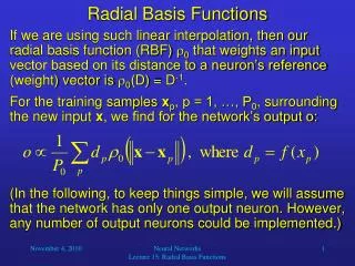
RBF network • This is becoming an increasingly popular neural network with diverse applications and is probably the main rival to the multi-layered perceptron • Much of the inspiration for RBF networks has come from traditional statistical pattern classification techniques
RBF network • The basic architecture for a RBF is a 3-layer network, as shown in Fig. • The input layer is simply a fan-out layer and does no processing. • The second or hidden layer performs a non-linear mapping from the input space into a (usually) higher dimensional space in which the patterns become linearly separable.
Output layer • The final layer performs a simple weighted sum with a linear output. • If the RBF network is used for function approximation (matching a real number) then this output is fine. • However, if pattern classification is required, then a hard-limiter or sigmoid function could be placed on the output neurons to give 0/1 output values.
Clustering • The unique feature of the RBF network is the process performed in the hidden layer. • The idea is that the patterns in the input space form clusters. • If the centres of these clusters are known, then the distance from the cluster centre can be measured. • Furthermore, this distance measure is made non-linear, so that if a pattern is in an area that is close to a cluster centre it gives a value close to 1.
Clustering • Beyond this area, the value drops dramatically. • The notion is that this area is radially symmetrical around the cluster centre, so that the non-linear function becomes known as the radial-basis function.
Gaussian function • The most commonly used radial-basis function is a Gaussian function • In a RBF network, r is the distance from the cluster centre. • The equation represents a Gaussian bell-shaped curve, as shown in Fig.
Distance measure • The distance measured from the cluster centre is usually the Euclidean distance. • For each neuron in the hidden layer, the weights represent the co-ordinates of the centre of the cluster. • Therefore, when that neuron receives an input pattern, X, the distance is found using the following equation:
Width of hidden unit basis function The variable sigma, , defines the width or radius of the bell-shape and is something that has to be determined empirically. When the distance from the centre of the Gaussian reaches , the output drops from 1 to 0.6.
Example • An often quoted example which shows how the RBF network can handle a non-linearly separable function is the exclusive-or problem. • One solution has 2 inputs, 2 hidden units and 1 output. • The centres for the two hidden units are set at c1 = 0,0 and c2 = 1,1, and the value of radius is chosen such that 22 = 1.
Example • The inputs are x, the distances from the centres squared are r, and the outputs from the hidden units are . • When all four examples of input patterns are shown to the network, the outputs of the two hidden units are shown in the following table.
x1 x2 r1 r2 1 2 0 0 0 2 1 0.1 0 1 1 1 0.4 0.4 1 0 1 1 0.4 0.4 1 1 2 0 0.1 1
Example • Next Fig. shows the position of the four input patterns using the output of the two hidden units as the axes on the graph - it can be seen that the patterns are now linearly separable. • This is an ideal solution - the centres were chosen carefully to show this result. • Methods generally adopted for learning in an RBF network would find it impossible to arrive at those centre values - later learning methods that are usually adopted will be described.
Training hidden layer • The hidden layer in a RBF network has units which have weights that correspond to the vector representation of the centre of a cluster. • These weights are found either using a traditional clustering algorithm such as the k-means algorithm, or adaptively using essentially the Kohonen algorithm.
Training hidden layer • In either case, the training is unsupervised but the number of clusters that you expect, k, is set in advance. The algorithms then find the best fit to these clusters. • The k -means algorithm will be briefly outlined. • Initially k points in the pattern space are randomly set.
Training hidden layer • Then for each item of data in the training set, the distances are found from all of the k centres. • The closest centre is chosen for each item of data - this is the initial classification, so all items of data will be assigned a class from 1 to k. • Then, for all data which has been found to be class 1, the average or mean values are found for each of co-ordinates.
Training hidden layer • These become the new values for the centre corresponding to class 1. • Repeated for all data found to be in class 2, then class 3 and so on until class k is dealt with - we now have k new centres. • Process of measuring the distance between the centres and each item of data and re-classifying the data is repeated until there is no further change – i.e. the sum of the distances monitored and training halts when the total distance no longer falls.
Adaptive k-means • The alternative is to use an adaptive k -means algorithm which similar to Kohonen learning. • Input patterns are presented to all of the cluster centres one at a time, and the cluster centres adjusted after each one. The cluster centre that is nearest to the input data wins, and is shifted slightly towards the new data. • This has the advantage that you don’t have to store all of the training data so can be done on-line.
Finding radius of Gaussians • Having found the cluster centres using one or other of these methods, the next step is determining the radius of the Gaussian curves. • This is usually done using the P-nearest neighbour algorithm. • A number P is chosen, and for each centre, the P nearest centres are found.
Finding radius of Gaussians • The root-mean squared distance between the current cluster centre and its P nearest neighbours is calculated, and this is the value chosen for . • So, if the current cluster centre is cj, the value is:
Finding radius of Gaussians • A typical value for P is 2, in which case is set to be the average distance from the two nearest neighbouring cluster centres.
XOR example • Using this method XOR function can be implemented using a minimum of 4 hidden units. • If more than four units are used, the additional units duplicate the centres and therefore do not contribute any further discrimination to the network. • So, assuming four neurons in the hidden layer, each unit is centred on one of the four input patterns, namely 00, 01, 10 and 11.
The P-nearest neighbour algorithm with P set to 2 is used to find the size if the radii. • In each of the neurons, the distances to the other three neurons is 1, 1 and 1.414, so the two nearest cluster centres are at a distance of 1. • Using the mean squared distance as the radii gives each neuron a radius of 1. • Using these values for the centres and radius, if each of the four input patterns is presented to the network, the output of the hidden layer would be:
input neuron 1 neuron 2 neuron 3 neuron 4 00 0.6 0.4 1.0 0.6 01 0.4 0.6 0.6 1.0 10 1.0 0.6 0.6 0.4 11 0.6 1.0 0.4 0.6
Training output layer • Having trained the hidden layer with some unsupervised learning, the final step is to train the output layer using a standard gradient descent technique such as the Least Mean Squares algorithm. • In the example of the exclusive-or function given above a suitable set of weights would be +1, –1, –1 and +1. With these weights the value of net and the output is:
input neuron 1 neuron 2 neuron 3 neuron 4 net output 00 0.6 0.4 1.0 0.6 –0.2 0 01 0.4 0.6 0.6 1.0 0.2 1 10 1.0 0.6 0.6 0.4 0.2 1 11 0.6 1.0 0.4 0.6 –0.2 0
Advantages/Disadvantages • RBF trains faster than a MLP • Another advantage that is claimed is that the hidden layer is easier to interpret than the hidden layer in an MLP. • Although the RBF is quick to train, when training is finished and it is being used it is slower than a MLP, so where speed is a factor a MLP may be more appropriate.
Summary • Statistical feed-forward networks such as the RBF network have become very popular, and are serious rivals to the MLP. • Essentially well tried statistical techniques being presented as neural networks. • Learning mechanisms in statistical neural networks are not biologically plausible – so have not been taken up by those researchers who insist on biological analogies.