Image matching using the Hausdorff Distance with CUDA
290 likes | 710 Views
Image matching using the Hausdorff Distance with CUDA. Ashish Shah. Hausdorff distance. set A = {a1,….,ap} and B = {b1,….,bq} - maximum distance of a set to the nearest point in the other set.

Image matching using the Hausdorff Distance with CUDA
E N D
Presentation Transcript
Image matching using the Hausdorff Distance with CUDA Ashish Shah
Hausdorff distance • set A = {a1,….,ap} and B = {b1,….,bq} - maximum distance of a set to the nearest point in the other set. - So in effect ranks each point of A based on its distance to the nearest point of B, and then uses the largest ranked such point as the distance - Hausdorff distance measures the amount of mismatch between two sets of points. - computed in O(pq(p+q)log(pq)) time
Minimal Hausdorff distance • Considers the mismatch between all possible relative positions of two sets • Minimal Hausdorff Distance MG defined as for all transformations(G) In the paper referred and project the focus is on the case where the relative position of the model with respect to the image is the group of translations
How to compute the MT In other words the H(A,B) can be computed by computing d(a) and d’(b) for all and Interested in the graph of d(x)which gives the distance from any point x to the nearest point in a set of source points in B
Voronoi surface It is a distance transform It defines the distance from any point x to the nearest of source points of the set A or B
Calculating Vornoi surfaceArray D [x,y] Algorithm • Process each row independently for each row calculate distance to nearest non-zero pixel in that row i.e. for each (x,y) it finds dx such that E[x+dx, y] or E[x-dx,y] is a non-zero pixel where dx is minimum non-negative number • Then scan each column up and down using the above computed dx values and using Euclidean norm calculate the nearest non-zero-pixel distance
Calculating Vornoi surfaceArray D [x,y] // x- KERNEL OVERVIEW for l = 0 to imagewidth if d[l] == infinity { for k = l+1 to imagewidth if d[k] == 0 distance = k - l for k = l-1 to 0 if d[k] == 0 && (l-k) < distance distance = l - k } d[l] = distance
Calculating Vornoi surfaceArray D [x,y] // y-KERNEL OVERVIEW for l = 0 to imageheight origdistance = d[l] distance = origdistance if d[l] != 0 { for k = l+1 to imageheight if (d[k] != infinity) && floord[k] == d[k] distance = k -l else geteuclideandistance(k-l, d[k]) for k = l-1 to 0 if d[k] != infinity && floord[k] == d[k] { tdistance = 0; if d[k] == 0 tdistance = l - k else tdistance = geteuclideandistance(l-k, d[k]) if tdistance < distance diatnce = tdistance } } d[l] = distance
Vornoi surfaceArray computation (nice to have) • Using Shared memory by cell decomposition technique • Verifying or comparing results by using Z-buffer for calculations, claims O(P) runtime in paper • Author states takes 1 sec to compute distance transform on Sun-4 (SPARC-2 machine) for 256x256 image, no results for bigger images, our results show considerable degradation for higher resolution images
Calculating Hausdorff distance array F [x,y] • Algorithm F[x,y] can be viewed as the maximization of distance transform D’[x,y] shifted by each location where model B[k,l] takes a nonzero value • Probing the Voronoi surface of the image • i.e. locations in the Voronoi surface of the image are probed and then F[x,y] is the maximum of these probe values for each position (x,y) of the model B[k,l].
Calculating Hausdorff distance array F [x,y] // hausdorffArrayKernel for k = 0 to modelheight for l = 0 to modelwidth element = M[l][k] * I[lx][ky] if (element > distance) { distance = element } d[o] = distance
Calculating Hausdorff distance array F [x,y] (nice to have) • Using shared memory with cell decomposition technique • Verifying technique with Z-buffer calculations, paper hasn’t verified this technique as well, mentions repeated Z-buffer loading could hamper the faster results as well • Efficient computation as described for CPU O(pq(p+q)logpq) • Ruling out circles • Early scan termination • Skipping forward • Mentions consideration between speedup methods important
Results extracted from paper (efficient computation) • Image: 360 x 240 pixels • Model: 115 x 199 pixels • Sun-4 (SPARCstation 2) Runtime ± 20 seconds • 2 matches Image model overlaid
Results from CUDA implementation • As per slide 15 - naïve approach - 256x256 image - 256x256 model - 13 seconds • Results show that for higher resolution images the timing doesn’t de-grade much wheras on CPU implementation suffers exponential degradation • Currently working on taking an actual binary image as input and doing a compare, planning on finishing implementation before end of project • Note this should have very little to no effect on our results reported
Comments • The method is quite tolerant of small position errors as occur with edge detectors and other feature extraction methods but a single outlier could throw the results off. • Partial Hausdorff Distance is the k-th ranked distance between a point and its nearest neighbor in the other set where distances are ranked in increasing order - nicely resistant to noise - need to figure out kth distance value Nice to do also: • Comparing multi-resolution image match techniques • Comparing images under rigid motion
References • References • [Huttenlocher et al., 1991]Huttenlocher Daniel P, Kedem K and M. SharirThe Upper Envelope of Voronoi Surfaces and Its Applications, ACM symposium on Computational Geometry,194-292, 1991 • Huttenlocher, D. P., Klanderman, G. A., and Rucklidge, W. A. 1993. Comparing Images Using the Hausdorff Distance. IEEE Trans. Pattern Anal. Mach. Intell. 15, 9 (Sep. 1993), 850-863. • Rucklidge, W. J. 1994 Efficient Computation of the Minimum Hausdorff Distance for Visual Recognition. Technical Report. UMI Order Number: TR94-1454., Cornell University.