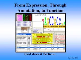
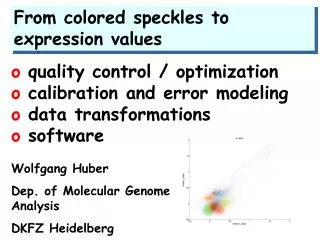
From colored speckles to expression values
From colored speckles to expression values. o quality control / optimization o calibration and error modeling o data transformations o software Wolfgang Huber Dep. of Molecular Genome Analysis DKFZ Heidelberg. samples: mRNA from tissue biopsies, cell lines. probes:

From colored speckles to expression values
E N D
Presentation Transcript
From colored speckles to expression values o quality control / optimizationo calibration and error modelingo data transformationso software Wolfgang Huber Dep. of Molecular Genome Analysis DKFZ Heidelberg
samples: mRNA from tissue biopsies, cell lines probes: gene-specific DNA strands detection tissue A tissue B tissue C ErbB2 0.02 1.12 2.12 VIM 1.1 5.8 1.8 ALDH4 2.2 0.6 1.0 CASP4 0.01 0.72 0.12 LAMA4 1.32 1.67 0.67 MCAM 4.2 2.93 3.31 microarrays
a microarray slide Slide: 25x75 mm 4x4 or 8x4 sectors 17...38 rows and columns per sector ca. 4600…46000 probes/array Spot-to-spot: ca. 150-350 mm sector: corresponds to one print-tip
Terminology sample: RNA (cDNA) hybridized to the array, aka target, mobile substrate. probe: DNA spotted on the array, aka spot, immobile substrate. sector: rectangular matrix of spots printed using the same print-tip (or pin) plate: set of 384 (768) spots printed with DNA from the same microtitre plate of clones slide,array channel: data from one color (Cy3 = cyanine 3 = green, Cy5 = cyanine 5 = red). batch: collection of microarrays with the same probe layout and quality
Image Analysis Raw data • scanner signal • 2D image: • 5 or 10 mm spatial resolution, • 16 bit (65536) dynamic range per channel • ca. 30-50 pixels per probe (60 mm spot size) • 40 MB per array spot intensities 2 numbers per probe (~100-300 kB) … auxiliaries: background, area, std dev, …
R and G for each spot on the array. Image analysis 1. Addressing. Estimate location of spot centers. 2. Segmentation. Classify pixels as foreground (signal) or background. • 3. Information extraction. For • each spot on the array and each • dye • foreground intensities; • background intensities; • quality measures.
Localbackground ---- GenePix ---- QuantArray ---- ScanAlyze
Affymetrix files Main software from Affymetrix: MAS - MicroArray Suite. DAT file: Image file, ~107 pixels, ~50 MB. CEL file: probe intensities, ~400k numbers CDF file: Chip Description File. Describes which probes go in which probe sets (genes, gene fragments, ESTs).
Affymetrix image analysis DAT image files CEL files Each probe cell: 10x10 pixels. Gridding: estimate location of cell centers. Signal: Remove outer 36 pixels 8x8 pixels. Probe cell signal, PM or MM, is the 75th percentile of the 8x8 pixel values. Background: Average of the lowest 2% probe cells is taken as the background value and subtracted. Compute also quality values.
Data and notation PMijg, MMijg= Intensity for perfect match and mismatch probe j for gene g in chip i. i = 1,…, n one to hundreds of chips j = 1,…, J usually 16 or 20 probe pairs g= 1,…, G 8…20,000 probe sets. Tasks: calibrate (normalize) the measurements from different chips (samples) summarize for each probe set the probe level data, i.e., 20 PM and MM pairs, into a single expression measure. compare between chips (samples) for detecting differential expression.
spot or probe intensity data n one-color arrays (Affymetrix, nylon) two-color spotted arrays Probes (genes) conditions (samples)
Spot intensities are not mRNA concentrations The point is not that these steps are ‘not perfect’; it is that they may vary from array to array, experiment to experiment.
Systematic Stochastic o similar effect on many measurements o corrections can be estimated from data o too random to be ex-plicitely accounted for o “noise” Calibration Error model Sources of variation amount of RNA in the biopsy efficiencies of -RNA extraction -reverse transcription -labeling -photodetection PCR yield DNA quality spotting efficiency, spot size cross-/unspecific hybridization stray signal
measured intensity of probe k in sample i unspecific gain actual abundance aik, bik all unknown: need to approximately determine from data
Implications quantity of interest data No non-linear terms: Saturation can be avoided in the experiments. Data from well-performed experiments shows no evidence for gross deviations from affine linearity. The flexibility (and complexity) lies in the number of parameters: twice the number of data points! parameters must not all be independent make simplifiying assumptions, reduce the number of independent parameters to manageable size Quality control: verify that assumptions hold for the data at hand Normalization, calibration: estimate parameters for the data at hand Error modeling: control the error bars both of measured yik and of estimated normalization parameters aik,bik
bi per-sample normalization factor bk sequence-wise labeling efficiency log hik ~ N(0,s22) “multiplicative noise” ai per-sample offset Lik local background provided by image analysis eik ~ N(0, bi2s12) “additive noise” A typical set of assumptions
Discussion and possible extensions Sequence-wise factors bkneed not be explicitely determined if only interested in relative expression levels The assumptions bring down the number of parameters to 2*d - the rest is modeled as noise. Array calibration terms ai, bi same for all probes on array - could extend to include print-tip or plate effects Probe affinities bk same for all arrays - could extend to include batch effects
Calibration = normalization =parameter estimation of model parameters o data heteroskedastic variance stabilizing data transformation o maximum likelihood estimator o model holds for genes that are unchanged; differentially transcribed genes act as outliers. o heavy-tailed data distributions robust variant of ML estimator, à la Least Trimmed Sum of Squares regression. o works up to breakdown point of 50%
Gene expression measures o average over multiple probes e.g. Affymetrix GeneChip MAS 4.0: trimmed mean o sort dj = PMj -MMj o exclude highest and lowest value o J := those pairs within 3 standard deviations of the average
Gene expression measures: MAS 5.0 Instead of MM, use "repaired" version CT CT = MM if MM<PM = PM / "typical log-ratio" if MM>=PM "Signal" = Tukey.Biweight (log(PM-CT)) (… median) Tukey Biweight: B(x) = (1 – x2/c2)2 if |x|<c, 0 otherwise
Expression measures: Li & Wong dChip fits a model for each gene where • qi: expression index for gene i • fj: probe sensitivity o estimate qi by maximum likelihood. o need at least 10 or 20 chips. Current version works with PMs only.
RMA method: Irizarry, Speed et al. (2002) o Estimate one global background value b=mode(MM). Otherwise ignore MM. o Assume: PM = Ytrue + b Estimate Y0 from PM and b as a conditional expectation E[strue|PM, b]. o Use log2(Y). o Nonparametric nonlinear calibration ('quantile normalization') across a set of chips.
RMA expression measures AvDiff – type: with A a set of “suitable” pairs. Li-Wong – type: robust estimation of ai: median polish (iterative: successively remove row and column medians and accumulate terms until the process stabilizes).
software www.bioconductor.org packages: affy Affymetrix pre-processing (CEL, CDF) marrayInput two-color slides vsn calibration and variance stabilization o open-source („reproducible research“) o based on R (biggest statistics library in the world)
Quality control verify the assumptions that underly the +calibration +error model visualization, diagnostic plots some examples what can go wrong
? Background usual assumption for spotted arrays: total brightness = specific part (from labeled sample cDNA) + background brightness (adjacent to spot)
0 Background usual assumption for Affymetrix arrays: PM intensity = + specific part (from labeled sample cDNA) MM intensity log(PM/MM) From: R. Irizarry et al., Biostatistics 2002
PCR plates Scatterplot, colored by PCR-plate Two RZPD Unigene II filters (cDNA nylon membranes)
spotting pin quality decline after delivery of 5x10⁵ spots after delivery of 3x10⁵ spots H. Sueltmann DKFZ/MGA
spatial effects R Rb R-Rbcolor scale by rank another array: print-tip color scale ~ log(G) color scale ~ rank(G) spotted cDNA arrays, Stanford-type
Batches: array to array differences dij = madk(hik -hjk) arrays i=1…63; roughly sorted by time
Coefficient of variation cDNA slide data from H. Sueltmann
Density representation of the scatterplot (76,000 clones, RZPD Unigene-II filters)
References Normalization for cDNA microarray data: a robust composite method addressing single and multiple slide systematic variation. YH Yang, S Dudoit, P Luu, DM Lin, V Peng, J Ngai and TP Speed. Nucl. Acids Res. 30(4):e15, 2002. Variance Stabilization Applied to Microarray Data Calibration and to the Quantification of Differential Expression. W.Huber, A.v.Heydebreck, H.Sültmann, A.Poustka, M.Vingron. Bioinformatics, Vol.18, Supplement 1, S96-S104, 2002. A Variance-Stabilizing Transformation for Gene Expression Microarray Data. BP Durbin, JS Hardin, DM Hawkins, DM Rocke. Bioinformatics, Vol.18, Suppl. 1, S105-110. Exploration, Normalization, and Summaries of High Density Oligonucleotide Array Probe Level Data. RA Irizarry, B Hobbs, F Collin, YD Beazer-Barclay, KJ Antonellis, U Scherf, TP Speed (2002). Biostatistics. http://biosun01.biostat.jhsph.edu/~ririzarr/papers/index.html A more complete list of references is in: Elementary analysis of microarray gene expression data. W. Huber, A. von Heydebreck, M. Vingron, manuscript. http://www.dkfz-heidelberg.de/abt0840/whuber/
Acknowledgements UMC Leiden Judith Boer Bioconductor Project Robert Gentleman Sandrine Dudoit Rafael Irizarry Laurent Gautier MPI Molekulare Genetik Anja von Heydebreck Martin Vingron Tim Beißbarth Uni Heidelberg Günther Sawitzki DKFZ Heidelberg Annemarie Poustka Holger Sültmann Frank Bergmann Andreas Buneß Katharina Finis Florian Haller Patrick Herde Yvonne Keßler Jörg Schneider Anke Schroth Klaus Steiner Stephanie Süß Markus Vogt Friederike Wilmer … and many more!