Download

1 / 84
860 likes | 1.49k Views
Logistic and Poisson Regression: Modeling Binary and Count Data LISA Short Course Series. Mark Seiss, Dept. of Statistics. Presentation Outline. 1. Introduction to Generalized Linear Models 2. Binary Response Data - Logistic Regression Model 3. Count Response Data -

E N D
Logistic and Poisson Regression: Modeling Binary and Count DataLISA Short Course Series Mark Seiss, Dept. of Statistics
Presentation Outline 1. Introduction to Generalized Linear Models 2. Binary Response Data - Logistic Regression Model 3. Count Response Data - Poisson Regression Model
Reference Material • Categorical Data Analysis – Alan Agresti • Examples found with SAS Code at www.stat.ufl.edu/~aa/cda/cda.html • Presentation and Data from Examples • www.stat.vt.edu/consult/short_courses.html
Generalized linear models (GLM) extend ordinary regression to non-normal response distributions. 3 Components Random – identifies response Y and its probability distribution Systematic – explanatory variables in a linear predictor function (Xβ) Link function – function (g(.)) that links the mean of the response (E[Yi]=μi) to the systematic component. Model for i = 1 to n Generalized Linear Models
Why do we use GLM’s? Linear regression assumes that the response is distributed normally GLM’s allow us to analyze the linear relationship between predictor variables and the mean of the response variable when it is not reasonable to assume the data is distributed normally. Generalized Linear Models
Predictor Variables Two Types: Continuous and Categorical Continuous Predictor Variables Examples – Time, Grade Point Average, Test Score, etc. Coded with one parameter – βixi Categorical Predictor Variables Examples – Sex, Political Affiliation, Marital Status, etc. Actual value assigned to Category not important Ex) Sex - Male/Female, M/F, 1/2, 0/1, etc. Coded Differently than continuous variables Generalized Linear Models
Categorical Predictor Variables cont. Consider a categorical predictor variable with L categories One category selected as reference category Assignment of Reference Category is arbitrary Variable represented by L-1 dummy variables Model Identifiability Two types of coding – Dummy and Effect Generalized Linear Models
Categorical Predictor Variables cont. Dummy Coding (Used in R) xk = 1 if predictor variable is equal to category k 0 otherwise xk = 0 for all k if predictor variable equals category I Effect Coding (Used in JMP) xk = 1 if predictor variable is equal to category k 0 otherwise xk = -1 for all k if predictor variable equals category I Generalized Linear Models
Saturated Model Contains a separate indicator parameter for each observation Perfect fit μ = y Not useful since there is no data reduction, i.e. number of parameters equals number of observations. Maximum achievable log likelihood – baseline for comparison to other model fits Generalized Linear Models
Deviance Let L(μ|y) = maximum of the log likelihood for the model L(y|y) = maximum of the log likelihood for the saturated model Deviance = D(y| μ) = -2 [L(μ|y) - L(y|y) ] Likelihood Ratio Statistic for testing the null hypothesis that the model is a good alternative to the saturated model Likelihood ratio statistic has an asymptotic chi-squared distribution with N – p degrees of freedom, where p is the number of parameters in the model. Allows for the comparison of one model to another using the likelihood ratio test. Generalized Linear Models
Nested Models Model 1 - model with p predictor variables {X1, X2, X3,….,Xp} and vector of fitted values μ1 Model 2 - model with q<p predictor variables {X1, X2, X3,….,Xq} and vector of fitted values μ2 Model 2 is nested within Model 1 if all predictor variables found in Model 2 are included in Model 1. i.e. the set of predictor variables in Model 2 are a subset of the set of predictor variables in Model 1 Model 2 is a special case of Model 1 - all the coefficients associated with Xp+1, Xp+2, Xp+3,….,Xq are equal to zero Generalized Linear Models
Likelihood Ratio Test Null Hypothesis: There is not a significant difference between the fit of two models. Null Hypothesis for Nested Models: The predictor variables in Model 1 that are not found in Model 2 are not significant to the model fit. Alternate Hypothesis for Nested Models - The predictor variables in Model 1 that are not found in Model 2 are significant to the model fit. Likelihood Ratio Statistic = -2* [L(y,u2)-L(y,u1)] = D(y,μ2) - D(y, μ1) Difference of the deviances of the two models Always D(y,μ2) > D(y,μ1) implies LRT > 0 LRT is distributed Chi-Squared with p-q degrees of freedom Generalized Linear Models
Likelihood Ratio Test cont. Later, we will use the Likelihood Ratio Test to test the significance of variables in Logistic and Poisson regression models. Generalized Linear Models
Theoretical Example of Likelihood Ratio Test 3 predictor variables – 1 Continuous (X1), 1 Categorical with 4 Categories (X2, X3, X4), 1 Categorical with 1 Category (X5) Model 1 - predictor variables {X1, X2, X3, X4, X5} Model 2 - predictor variables {X1, X5} Null Hypothesis – Variables with 4 categories is not significant to the model (β2 = β3 = β4= 0) Alternate Hypothesis - Variable with 4 categories is significant Likelihood Ratio Statistic = D(y,μ2) - D(y, μ1) Difference of the deviance statistics from the two models Chi-Squared Distribution with 5-2=3 degrees of freedom Generalized Linear Models
Model Selection 2 Goals: Complex enough to fit the data well Simple to interpret, does not overfit the data Study the effect of each predictor on the response Y Continuous Predictor – Graph P[Y=1] versus X Discrete Predictor - Contingency Table of P[Y=1] versus categories of X Unbalance Data – Few responses of one type Guideline – 10 outcomes of each type for each X terms Example – Y=1 for only 30 observations out of 1000 Model should contain no more than 3 X terms Generalized Linear Models
Model Selection cont. Multicollinearity Correlations among predictors resulting in an increase in variance Reduces the significance value of the variable Occurs when several predictor variables are used in the model Determining Model Fit Other criteria besides significance tests (i.e. Likelihood Ratio Test) can be used to select a model Generalized Linear Models
Model Selection cont. Determining Model Fit cont. Akaike Information Criterion (AIC) Penalizes model for having many parameters AIC = Deviance+2*p where p is the number of parameters in model Bayesian Information Criterion (BIC) BIC = -2 Log L + ln(n)*p where p is the number of parameters in model and n is the number of observations Generalized Linear Models
Model Selection cont. Selection Algorithms Best subset – Tests all combinations of predictor variables to find best subset Algorithmic – Forward, Backward and Stepwise Procedures Generalized Linear Models
Best Subsets Procedure Run model with all possible combinations of the predictor variables Number of possible models equal to 2p where p is the number of predictor variables Dummy Variables for categorical predictors considered together Ex) For a set of predictors {X1, X2, X3} runs models with sets of predictors {X1, X2, X3}, {X1, X2}, {X2, X3}, {X1, X3}, {X1}, {X2}, {X3}, and no predictor variables. 23 = 8 possible models Most programs only allow for a small set of predictor variables Cannot be run in a reasonable amount of time 210 = 1024 models run for a set of 10 predictor variables Generalized Linear Models
Forward Selection Idea: Start with no variables in the model and add one at a time Step One: Fit model with single predictor variable and determine fit Step Two: Select predictor variable with best fit and add to model Step Three: Add each variable to the model one at a time and determine fit Step Four: If at least one variable produces better fit, return to step two If no variables produce better fit, use model Drawback: Variables Added to the model cannot be taken out. Generalized Linear Models
Backward Selection Idea: Start with all variables in the model and take out one at a time Step One: Fit all predictor variables in model and determine fit Step Two: Delete one variable at a time and determine fit Step Three: If the deletion of at least one variable produces better fit, remove variable that produces best fit when deleted and return to step 2 If the deletion of a variable does not produce a better fit, use model Drawback: Variables taken out of model cannot be added back in. Generalized Linear Models
Stepwise Selection Idea: Combination of forward and backward selection Forward Step then backward step Step One: Fit each predictor variable as a single predictor variable and determine fit Step Two: Select variable that produces best fit and add to model. Step Three: Add each predictor variable one at a time to the model and determine fit Step Four: Select variable that produces best fit and add to the model Step Five: Delete each variable in the model one at a time and determine fit Step Six: Remove variable that produces best fit when deleted Step Seven: Return to Step Two Loop until no variables added or deleted improve the fit. Generalized Linear Models
Summary 3 Components of the GLM Random (Y) Link Function (g(E[Y])) Systematic (xtβ) Continuous and Categorical Predictor Variables Coding Categorical Variables – Effect and Dummy Coding Likelihood Ratio Test for Nested Models Test the significance of a predictor variable or set of predictor variables in the model. Model Selection – Best Subset, Forward, Backward, Stepwise Generalized Linear Models
Questions/Comments Generalized Linear Models
Consider a binary response variable. Variable with two outcomes One outcome represented by a 1 and the other represented by a 0 Examples: Does the person have a disease? Yes or No Who is the person voting for? McCain or Obama Outcome of a baseball game? Win or loss Logistic Regression
Logistic Regression Example Data Set Response Variable –> Admission to Grad School (Admit) 0 if admitted, 1 if not admitted Predictor Variables GRE Score (gre) Continuous University Prestige (topnotch) 1 if prestigious, 0 otherwise Grade Point Average (gpa) Continuous Logistic Regression
First 10 Observations of the Data Set ADMIT GRE TOPNOTCH GPA 1 380 0 3.61 0 660 1 3.67 0 800 1 4 0 640 0 3.19 1 520 0 2.93 0 760 0 3 0 560 0 2.98 1 400 0 3.08 0 540 0 3.39 1 700 1 3.92 Logistic Regression
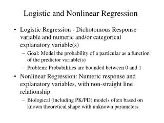
Consider the linear probability model where yi = response for observation i xi = 1x(p+1) matrix of covariates for observation i p = number of covariates GLM with binomial random component and identity link g(μ) = μ Issue: π(Xi) can take on values less than 0 or greater than 0 Issue: Predicted probability for some subjects fall outside of the [0,1] range. Logistic Regression
Consider the logistic regression model GLM with binomial random component and identity link g(μ) = logit(μ) Range of values for π(Xi) is 0 to 1 Logistic Regression
Consider the logistic regression model And the linear probability model Then the graph of the predicted probabilities for different grade point averages: Important Note: JMP models P(Y=0) and effect coding is used for categorical variables Logistic Regression
Interpretation of Coefficient β – Odds Ratio The odds ratio is a statistic that measures the odds of an event compared to the odds of another event. Say the probability of Event 1 is π1and the probability of Event 2 is π2. Then the odds ratio of Event 1 to Event 2 is: Value of Odds Ratio range from 0 to Infinity Value between 0 and 1 indicate the odds of Event 2 are greater Value between 1 and infinity indicate odds of Event 1 are greater Value equal to 1 indicates events are equally likely Logistic Regression
Interpretation of Coefficient β – Odds Ratio cont. Link to Logistic Regression : Thus the odds ratio between two events is Logistic Regression
Interpretation of Coefficient β – Odds Ratio cont. Consider Event 1 is Y=0 given X and Event 2 is Y=0 given X+1 From our logistic regression model Thus the ratio of the odds of Y=0 for X and X+1 is Logistic Regression
Single Continuous Predictor Variable - GPA Generalized Linear Model Fit Response: Admit Modeling P(Admit=0) Distribution: Binomial Link: Logit Observations (or Sum Wgts) = 400 Whole Model Test Model -LogLikelihood L-R ChiSquare DF Prob>ChiSq Difference 6.50444839 13.0089 1 0.0003 Full 243.48381 Reduced 249.988259 Goodness Of Fit Statistic ChiSquare DF Prob>ChiSq Pearson 401.1706 398 0.4460 398 0.4460 Deviance 486.9676 398 0.0015 398 0.0015 Logistic Regression
Single Continuous Predictor Variable – GPA cont. Effect Tests Source DF L-R ChiSquare Prob>ChiSq GPA 1 13.008897 0.0003 Parameter Estimates Term Estimate Std Error L-R ChiSquare Prob>ChiSq Lower CL Upper CL Intercept -4.357587 1.0353175 19.117873 <.0001 -6.433355 -2.367383 GPA 1.0511087 0.2988695 13.008897 0.0003 0.4742176 1.6479411 Interpretation of the Parameter Estimate: Exp{1.0511087} = 2.86 = odds ratio between the odds at x+1 and odds at x for all x The ratio of the odds of being admitted between a person with a 3.0 gpa and 2.0 gpa is equal to 2.86 or equivalently the odds of the person with the 3.0 is 2.86 times the odds of the person with the 2.0. Logistic Regression
Single Categorical Predictor Variable – Top Notch Generalized Linear Model Fit Response: Admit Modeling P(Admit=0) Distribution: Binomial Link: Logit Observations (or Sum Wgts) = 400 Whole Model Test Model -LogLikelihood L-R ChiSquare DF Prob>ChiSq Difference 3.53984692 7.0797 1 0.0078 Full 246.448412 Reduced 249.988259 Goodness Of Fit Statistic ChiSquare DF Prob>ChiSq Pearson 400.0000 398 0.4624 Deviance 492.8968 398 0.0008 I Logistic Regression
Single Categorical Predictor Variable – Top Notch cont. Effect Tests Source DF L-R ChiSquare Prob>ChiSq TOPNOTCH 1 7.0796939 0.0078 Parameter Estimates Term Estimate Std Error L-R ChiSquare Prob>ChiSq Lower CL Upper CL Intercept -0.525855 0.138217 14.446085 0.0001 -0.799265 -0.255667 TOPNOTCH[0] -0.371705 0.138217 7.0796938 0.0078 -0.642635 -0.099011 Interpretation of the Parameter Estimate: Exp{2*-.371705} = 0.4755 = odds ratio between the odds of admittance for a student at a less prestigous university and the odds of admittance for a student from a more prestigous university. The odds of being admitted from a less prestigous university is .48 times the odds of being admitted from a more prestigous university. I Logistic Regression
Variable Selection– Likelihood Ratio Test Consider the model with GPA, GRE, and Top Notch as predictor variables Generalized Linear Model Fit Response: Admit Modeling P(Admit=0) Distribution: Binomial Link: Logit Observations (or Sum Wgts) = 400 Whole Model Test Model -LogLikelihood L-R ChiSquare DF Prob>ChiSq Difference 10.9234504 21.8469 3 <.0001 Full 239.064808 Reduced 249.988259 Goodness Of Fit Statistic ChiSquare DF Prob>ChiSq Pearson 396.9196 396 0.4775 Deviance 478.1296 396 0.0029 Logistic Regression
Variable Selection– Likelihood Ratio Test cont. Effect Tests Source DF L-R ChiSquare Prob>ChiSq TOPNOTCH 1 2.2143635 0.1367 GPA 1 4.2909753 0.0383 GRE 1 5.4555484 0.0195 Parameter Estimates Term Estimate Std Error L-R ChiSquare Prob>ChiSq Lower CL Upper CL Intercept -4.382202 1.1352224 15.917859 <.0001 -6.657167 -2.197805 TOPNOTCH[0] -0.218612 0.1459266 2.2143635 0.1367 -0.503583 0.070142 GPA 0.6675556 0.3252593 4.2909753 0.0383 0.0356956 1.3133755 GRE 0.0024768 0.0010702 5.4555484 0.0195 0.0003962 0.0046006 Logistic Regression
Model Selection – Forward Stepwise Fit Response: Admit Stepwise Regression Control Prob to Enter 0.250 Prob to Leave 0.100 Direction: Rules: Current Estimates -LogLikelihood RSquare 239.06481 0.0437 Logistic Regression
Model Selection – Forward cont. Parameter Estimate nDF Wald/Score ChiSq "Sig Prob" Intercept[1] -4.3821986 1 0 1.0000 GRE 0.00247683 1 5.356022 0.0207 GPA 0.66755511 1 4.212258 0.0401 TOPNOTCH{1-0} 0.21861181 1 2.244286 0.1341 Step History Step Parameter Action L-R ChiSquare "Sig Prob" RSquare p 1 GRE Entered 13.92038 0.0002 0.0278 2 2 GPA Entered 5.712157 0.0168 0.0393 3 3 TOPNOTCH{1-0} Entered 2.214363 0.1367 0.0437 4 Logistic Regression
Model Selection – Backward Start by selecting to enter all variables into the model Stepwise Fit Response: Admit Stepwise Regression Control Prob to Enter 0.250 Prob to Leave 0.100 Direction: Backward Rules: Combine Logistic Regression
Model Selection – Backward cont. Current Estimates -LogLikelihood RSquare 240.17199 0.0393 Parameter Estimate nDF Wald/Score ChiSq "Sig Prob" Intercept[1] -4.9493751 1 0 1.0000 GRE 0.00269068 1 6.473978 0.0109 GPA 0.75468641 1 5.576461 0.0182 TOPNOTCH{1-0} 0 1 2.259729 0.1328 Step History Step Parameter Action L-R ChiSquare "Sig Prob" RSquare p 1 TOPNOTCH{1-0} Removed 2.214363 0.1367 0.0393 3 Logistic Regression
Variable Selection – Stepwise Stepwise Fit Response: Admit Stepwise Regression Control Prob to Enter 0.250 Prob to Leave 0.250 Direction: Mixed Rules: Combine Current Estimates -LogLikelihood RSquare 239.06481 0.0437 Logistic Regression
Variable Selection – Stepwise cont. Parameter Estimate nDF Wald/Score ChiSq "Sig Prob" Intercept[1] -4.3821986 1 0 1.0000 GRE 0.00247683 1 5.356022 0.0207 GPA 0.66755511 1 4.212258 0.0401 TOPNOTCH{1-0} 0.21861181 1 2.244286 0.1341 Step History Step Parameter Action L-R ChiSquare "Sig Prob" Rsquare p 1 GRE Entered 13.92038 0.0002 0.0278 2 2 GPA Entered 5.712157 0.0168 0.0393 3 3 TOPNOTCH{1-0} Entered 2.214363 0.1367 0.0437 4 Logistic Regression
Summary Introduction to the Logistic Regression Model Interpretation of the Parameter Estimates β – Odds Ratio Variable Significance – Likelihood Ratio Test Model Selection Forward Backward Stepwise Logistic Regression
Questions/Comments Logistic Regression
Consider a count response variable. Response variable is the number of occurrences in a given time frame. Outcomes equal to 0, 1, 2, …. Examples: Number of penalties during a football game. Number of customers shop at a store on a given day. Number of car accidents at an intersection. Poisson Regression
Poisson Regression Example Data Set Response Variable –> Number of Days Absent – Integer Predictor Variables Gender- 1 if Female, 2 if Male Ethnicity – 6 Ethnic Categories School – 1 if School, 2 if School 2 Math Test Score – Continuous Language Test Score – Continuous Bilingual Status – 6 Bilingual Categories Poisson Regression