Extending Dependencies with Conditions
280 likes | 679 Views
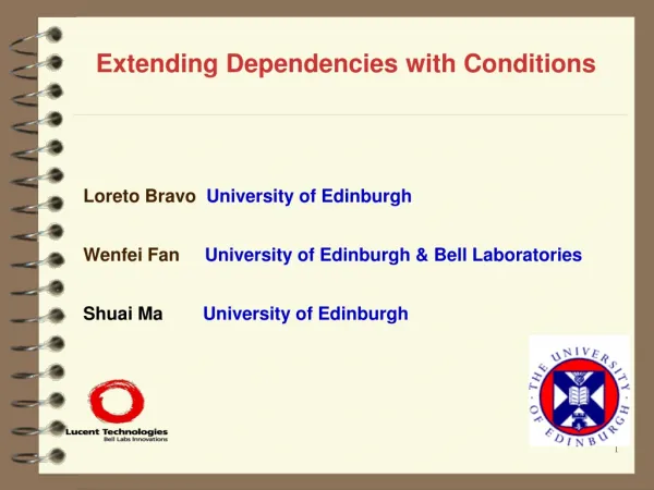
Extending Dependencies with Conditions. Loreto Bravo University of Edinburgh Wenfei Fan University of Edinburgh & Bell Laboratories Shuai Ma University of Edinburgh. Outline. Why Conditional Dependencies? Data Cleaning Schema Matching

Extending Dependencies with Conditions
E N D
Presentation Transcript
Extending Dependencies with Conditions Loreto Bravo University of Edinburgh Wenfei Fan University of Edinburgh & Bell Laboratories Shuai Ma University of Edinburgh
Outline • Why Conditional Dependencies? • Data Cleaning • Schema Matching • Conditional Inclusion Dependencies (CINDs) • Definition • Static Analysis • Satisfiability Problem • Implication Problem • Inference System • Static Analysis of CFDs+CINDs • Satisfiability Checking Algorithms (CFDs+CINDs) • Summary and Future Work
Motivation • Data Cleaning • Real life data is dirty! • Specify consistency using integrity constraints • Inconsistencies emerge as violations of constraints • Constraints considered so far: traditional • Functional Dependencies - FD • Inclusion Dependencies - IND • . . . • Schema matching: needed for data exchange and data integration • Pairings between semantically related source schema attributes and target schema attributes • expressed as inclusion dependencies (e.g., Clio)
Example: Amazon database • Schema: • book(id, isbn, title, price, format) • CD(id, title, price, genre) • order(id, title, type, price, country, county) CD book order
Data cleaning with inclusion dependencies • Example Inclusion dependency: • book[id, title, price] order[id, title, price] • Definition of Inclusion Dependencies (INDs) • R1[X] R2[Y], for any tuple t1 in R1, there must exist a tuple t2 in R2, such that t2[Y]=t1[X] book order
Data cleaning meets conditions This inclusion dependency does not make sense! • How to express? • Every book in order table must also appear in book table • Traditional inclusion dependencies: • order[id, title, price] book[id, title, price] order book
Data cleaning meets conditions • Conditional inclusion dependency: • order[id, title, price, type =‘ book’] book[id, title, price] order book
Schema matching with inclusion dependencies • Traditional inclusion dependencies: book[id, title, price] order[id, title, price] CD[id, title, price] order[id, title, price] • Schema Matching: • Pairings between semantically related source schema attributes and target schema attributes, which are de facto inclusion dependencies from source to target (e.g., Clio) order book CD
Schema matching meets conditions • Traditional inclusion dependencies: order[id, title, price] book[id, title, price] order[id, title, price] CD[id, title, price] These inclusion dependencies do not make sense! order book CD
Schema matching meets conditions order book CD Conditional inclusion dependencies: order[id, title, price; type =‘ book’] book[id, title, price] order[id, title, price; type = ‘CD’] CD[id, title, price] The constraints do not hold on the entire order table • order[id, title, price] book[id, title, price]holds only if type = ‘book’ • order[id, title, price] CD[id, title, price]holds only if type = ‘CD’
Conditional Inclusion Dependencies (CINDs) • (R1[X; Xp] R2[Y; Yp], Tp): • R1[X] R2[Y]: embedded traditional IND from R1 to R2 • attributes: X Xp Y Yp • Tp: a pattern tableau • tuples in Tp consist of constants and unnamed variable _ • Example: CD[ id, title, price; genre = ‘a-book’] book[ id, title, price; format = ‘audio’] • Corresponding CIND: • (CD[id, title, price; genre] book[id, title, price; format], Tp) Tp
INDs as a special case of CINDs R1[X] R2[Y] • X: [A1, …, An] • Y : [B1, …, Bn] As a CIND: (R1[X; nil] R2[Y; nil], Tp) • pattern tableau Tp: a single tuple consisting of _ only CINDs subsume traditional INDs
Static Analysis of CINDs • Satisfiability problem • INPUT: Give a set Σ of constraints • Question: Does there exist a nonempty instance I satisfying Σ? • Whether Σ itself is dirty or not • For INDs the problem is trivially true • For CFDs (to be seen shortly) it is NP-complete • Good news for CINDs Proposition: Any set of CINDs is always satisfiable I╠Σ
Static Analysis of CINDs • Implication problem • INPUT: set Σ of constraints and a single constraint φ • Question: for each instance I thatsatisfies Σ, doesIalsosatisfy φ? • Remove redundant constraints • PSPACE-complete for traditional inclusion dependencies Theorem. Complexity bounds for CINDs • Presence of constants • PSPACE-complete in the absence of finite domain attributes • Good news – The same as INDs • EXPTIME-complete in the general setting Σ╠φ
Finite axiomatizability of CINDs 1-Reflexivity 2-Projection and Permutation 3-Transitivity • φ is implied by Σ iff it can be computed by the inference system • INDs have such Inference System • Good news: CINDs too! IND Counterparts Sound and Complete in the Absence of Finite Attributes 4-Downgrading 5-Augmentation 6-Reduction 7-F-reduction 8-F-upgrade Finite Domain Attributes Theorem. The above eight rules constitute a sound and complete inference system for implication analysis of CINDs
New CINDs can be inferred by axioms (R1[X; A] R2[Y; Yp], Tp), dom(A) = { true, false} Axioms for CINDs: finite domain reduction Tp then (R1[X; Xp] R2[Y; Yp], tp),
Static analyses: CIND vs. IND • In the absence of finite-domain attributes: • General setting with finite-domain attributes: CINDs retain most complexity bounds of their traditional counterpart
Conditional Functional Dependencies (CFDs) An extension of traditional FDs Example:cust([country = 44, zip] [street])
Static analyses: CFD + CIND vs. FD + IND • CINDs and CFDs properly subsume FDs and INDs • Both the satisfiability analysis and implication analysis are beyond reach in practice This calls for effective heuristic methods
Satisfiability Checking Algorithms • Before using a set of CINDs for data cleaning or schema matching we need to make sure that they make sense (that they are clean) • We need to find heuristics to solve the satisfiability problem • Input: A set Σ of CFDs and CINDs • Output: true / false • We modified and extended techniques used for FDs and INDs • For example: Chase, to builda “canonical” witness instance, i.e.,I╠Σ
= {1, ψ1} 1=(R2(G → H), (_ || c)) - CFD ψ1=(R2[G; nil] R1[F; nil], (_ || _) ) - CIND ChaseCFDs+CINDs – Terminate case R1 R2 R1 R2 1 ψ1 R1 R2 Done!
= {1, ψ1, ψ2} 1=(R2(G → H), (_ || c)) - CFD ψ1=(R2[G; nil] R1[F; nil], (_ || _) ) - CIND ψ2=(R1[E; nil] R2[G; nil], (_ || _) ) ChaseCFDs+CINDs – Loop case R1 R2 R1 R2 ψ1 ψ1 ψ2 Infinite application of ψ1 and ψ2 Loop! ψ2
More about the checking algorithms • Simplification of the chase: • The fresh variables are taken from a finite set • We avoid the infinite loop of the chase by limiting the size of the witness instance • If the algorithm returns: • True: we know the constraints are satisfiable • False: there may be false negative answers – the problem is undecidable and the best we can get is a heuristic • In order to improve accuracy of the algorithm we use: • Optimization techniques
Ψ2, Ψ3 Ψ4 Ψ5 R6 R3 R1 R2 R5 R4 Ψ1 Example optimization techniques Unsatisfiability Propagation • IF • CFDs on R4 is unsatisfiable • There is a CIND Ψ4: (R3[X; nil] R4[Y; Yp], tp) • THEN • R3 must be empty! Node(Relation): related to CFDs Edge: related to CINDS
CFDs+CINDs satisfiabilitychecking - experiments • Experimental Settings • Accuracy tested for satisfiable sets of CFDs and CINDs • The data sets where generated by ensuring the existence of a witness database that satisfies them • Scalability tested for random sets of CFDs and CINDs • Each experiment was run 6 times and the average is reported • # of constraints: up to 20,000 • # of relations: up to 100 • Ratio of finite attributes: up to 25% • An Intel Pentium D 3.00GHz with 1GB memory
CFDs+CINDs satisfiabilitychecking - experiments Algorithm: 1. Chase : modified version Chase 2. DG+Chase: graph optimization based Chase Accuracy testing is based satisfiable sets of CFDs and CINDs
CFDs+CINDs satisfiabilitychecking - experiments Scalability testing is based on random sets of CFDs and CINDs
Summary and future work • New constraints: conditional inclusion dependencies • for bothdata cleaning and schema matching • complexity bounds of satisfiability and implication analyses • a sound and complete inference system • Complexity bounds for CFDs and CINDs taken together • Heuristic satisfiabilitychecking algorithms for CFDs and CINDs • Open research issues: • Deriving schema mapping from the constraints • Repairing dirty data based on CFDs + CINDs • Discovering CFDs + CINDs Towards a practical method for data cleaning and schema matching