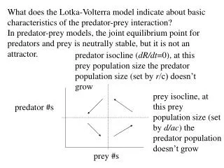
What does the Lotka-Volterra model indicate about basic characteristics of the predator-prey interaction?

1. What does the Lotka-Volterra model indicate about basic characteristics of the predator-prey interaction? In predator-prey models, the joint equilibrium point for predators and prey is neutrally stable, but it is not an attractor. predator isocline (dR/dt=0), at this prey population size the predator population size (set by r/c) doesn’t grow prey isocline, at this prey population size (set by d/ac) the predator population doesn’t grow predator #s prey #s

2. The isoclines define regions where prey grow or decline in numbers, and similarly for predators. Above the predator isocline, predator numbers can grow; below it predator numbers decrease. predator isocline predators prey

3. On this copy of the diagram, you can see that when predator numbers are lower than the prey isocline, prey can increase; when above, prey numbers decrease. predators prey isocline prey

4. How do cycles change when either r or c is changed? Remember: Peq = r/c Req = d/ac The prey isocline is set by r/c. If r increases or c decreases, the prey isocline rises. The equilibrium, based on prey growth rate and predator capture efficiency, “can stand” more predators. The predator population grows to this isocline. This does not pull the populations back toward the common stable point! If the death rate of predators, d, increased and/or either (or both) c or a decreased, the predator isocline would move right, and the number of prey could increase up to the isocline. This doesn’t move the populations back toward the stable point either!

5. Changing the parameters “de-stabilizes” the interaction. • Changing the determining parameters (d, a, c, r) can, like the effect of increasing growth during lags in logistic growth, cause the amplitude of cycles in predators and prey to increase (it also changes the period of the cycles), and makes the extinction of one (or both) species more likely. • Reviewing the output you should have seen from Populus… • 1. “Standard cycles” – Predators: P0 =20, r2 = 0.1, C = 0.01 • Prey: N0 = 20, r1 = 0.1, C = 0.01

7. Increasing the value of c, the capture (or encounter) efficiency causes the amplitude of the prey cycle to increase, but the portion of the cycle at low abundance to increase a lot, and can result in extinction… Change parameters for the prey to N0 = 20, r = 0.1, c = 0.05 prey predator

8. The increase in c created a predator that overexploited its prey. In this model the prey declines to very low number for quite a while, until the predator population had reached very small numbers for a time. Do predators overexploit their prey in nature (and cause their extinction)? (Think here of the Red Queen argument. Is this likely to occur in co-evolved natural populations? Extremely rarely in nature, but when it happens, it usually involves the introduction (by chance or human activity) of an exotic predator that had not evolved in conjunction with the overexploited prey.

9. One example: Humans, thinking they could increase the biomass of fish that could be harvested from African rift lakes (Victoria, Tanganyika, Malawi), introduced Nile perch into Lake Victoria. Of >300 species of endemic cichlid fish in Lake Victoria, more than 200 were driven extinct by the perch. This represents the largest mass extinction of the modern era. Local fisherman can now harvest less.

10. The basic Lotka-Volterra model can generate extinction, rather than just low values. Now let’s try increasing the value of c from 0.01 (initially) to 0.1 (an increase of a factor of 10…

11. Back to predator – prey cycles… There are good examples of cycles without the heavy interference of the experimenter. They support the basic Lotka-Volterra model of cycles. One good one involves the interaction of the azuki bean weevil and its braconid wasp parasite.

12. Here are the ‘steps’ in this cycle: (The weevils got a constant ration of seeds.) 1. The weevils grow toward a carrying capacity determined by the size of the ration. 2. The wasp population, once introduced, increases rapidly; wasp parasitism becomes a major source of mortality for weevils. 3. The weevil population declines. 4. Wasps are very (but not perfectly) efficient parasites, and continue to reduce the population of weevils. 5. When the weevil population nears extinction, there is insufficient food for the wasps; their population decreases rapidly. 6. Now weevil larvae that were not parasitized can increase and begin a new cycle.

13. When we compare theory to predator-prey interactions in the field (N.B. not lab environments), what are the differences? One key difference is that there are refuges in nature. The more efficient the predator, the more important refuges are.

14. Another important question: Do predator-prey cycles occur in natural ecosystems? • Answer: Only very rarely. • However there are examples (though qualification is necessary; these are the only examples I could think of). Here are a couple: • Cycles in the populations of arctic lemmings and their predators, the snowy owl. The necessary qualification is very similar to one that will arise in explaining example 2. • Cycles in the populations of arctic hares and their predator, the lynx. This is the example usually cited, due to the long record of fur purchases (~1710 - ~1960) kept by the Hudson Bay Company.

15. Here is the part of that more than 200 year record shown in textbooks: Note the scales on the two Y axes. And here are the participants interacting:

16. The period of the cycle is ~10 years. We expect that if we were to plot relative densities of predator and prey on Y and X axes respectively, with different points representing different times in a cycle, theory says that the points should move counterclockwise. However, when Gilpin did this, he got: Lynx

17. If the cycles are running backwards, do hares eat lynx? • Not likely! • Gilpin (and others) had explanative suggestions: • The hares might serve as reservoirs of diseases transmitted to lynx. • Trappers may have waited until hare numbers were high before going out to trap either species. That would make peaks appear to be nearly simultaneous (as they appear) or even show lynx ‘leading’ hares. Recent scientific counts suggest that this trapping bias may have occurred. • Krebs et al. (1995) showed that food quality for the hares may be a key factor in explaining their cycles, and thus that lynx are simply following along. Here is how it works:

18. Hare number increases. • Larger number means lower food abundance and quality • left for hares to eat. • C. Hares lose weight, juvenile mortality increases, and the • now extended foraging time necessary to find food • increases exposure to predators. Hare numbers decrease. • D. The plant community begins to recover, but the first plants • to increase in abundance are toxic to hares. Toxins have • been identified, but they do not appear until after the hare • population declines. • E. The plant community completes recovery while the hares • remain at low density. • F. Then, with non-toxic plant biomass increased, the hare • population once more increases.

19. So, what the the toxic plants can do is slow the recovery of the hare population. Further, the lynx can also slow recovery during harsh winters. However, most of the time, the evidence suggests that the lynx does not ‘cause’ hare cycles, but the size of the lynx population simply ‘tracks’ the abundance of hares. What this shows is a modern view of interactive effects in the form of cascades. Modern ecology frequently also asks the question of whether controlling influences work ‘bottom- up’, i.e. the food is the ultimate control, or ‘top-down’, which would assign basic control to the lynx.

20. It is worth noting, though they will not be considered here, that there are alternatives to the Lotka-Volterra model, e.g. the Nicholson-Bailey model for parasite – host interaction. You have or will, depending on how far in advance (or after your scheduled lab) you do lab exercises, explore the Nicholson – Bailey model this week.

21. One of the problems that led to the development of alternative models is the lack of any aspect of predator behaviour. The model, with fixed c, assumes that the predator does not respond behaviourally to changes in the size and availability of the prey population. • Real predators respond in two ways to changes in prey abundance: • A numerical response, and • A functional response

22. Numerical response Numerical responses occur in many predator populations. Here is an approximate curve describing the type of response C.S. Holling observed using shrews as predators: Number of predators Number of prey

23. Another kind of numerical response: In short-eared owls, there is variation in clutch size depending on the abundance of prey. In the field, clutch sizes range from 4 (in ‘poor’ years) to 7 (in years of high prey abundance. In addition to a response in reproduction, there can be immigration to areas of high prey abundance. In Alaska…

24. Functional responses are more complicated. These responses are the result of the hunting behaviour of individual predators. The functional response is determined by the pattern of consumption of prey as the abundance of those prey increases. Specifically, it is the number of prey eaten per predator, as prey numbers increase. There are 3 patterns into which functional responses are usually grouped…

25. TYPE I FUNCTINAL REPSONSE This is the response of a filter feeding predator, e.g. a baleen whale. As prey (krill) abundance increases, the swimming of the whale through the higher density of krill increases the number of prey eaten in direct proportion to prey abundance. However, at some abundance of prey, the filter is filled, and more prey can’t be taken. Here’s what the relationship looks like…

26. TYPE II FUNCTIONAL RESPONSE This type of functional response was observed by Holling in studies of sawflies. It is common among invertebrate predators. The shape of the curve is determined by the characteristics of the predator in searching for, handling and eating prey. As prey become more numerous, the predator has to spend a greater fraction of its time in handling and eating, leaving less time for searching. At some density, a balance is reached, and more prey can’t be taken.

27. TYPE III FUNCTIONAL RESPONSE This response is seen in higher vertebrates and some higher invertebrates. The curve shows that the predator is ‘switching’ from some other prey when this one is scarce to a high capture rate for this prey when it is more common. Note that at high prey density this looks very much like the type II response.

28. What might cause a type III response? • Habitat heterogeneity, with refuges available. Prey achieve safety in refuges, but, as population size increases, there are not enough refuges for all prey. • Predators form ‘search images’ that aid in prey capture. At low prey abundance, the search images may not be reinforced. Capture is less efficient. • Finding sufficient food when this prey is scarce may force the predator to ‘switch’ to more abundant alternatives. • There is lots of experimental evidence of this switching behaviour in predators. The text shows you an invertebrate example…

30. Your text also shows you a view of these functional responses that explains the potential of the predator population to limit (or regulate) the size of the prey population… Note the different y-axes of the two graphs: number and proportion of prey consumed.

31. To expand on the theoretical view of functional responses, here’s evidence of a real functional response (Pentatomid ‘bug’ attacking a sawfly larval stage) plotted as prey/predator against prey density. The curve has a clear ‘hump’.

32. Type I predators consume a constant proportion of the prey population (until satiation is reached; at abundances above that they take a declining proportion of the total prey). Type II predators take a declining proportion of the prey as prey abundance increases. That clearly cannot limit (or regulate) the prey. However, type III predators can, if they are efficient enough, limit the prey population. It is at an intermediate prey abundance that the proportion of prey captured is maximum. Only type III has this maximum.

33. A type III predator functional response can increase the likelihood of predator and prey persistence. What tends to reduce the amplitude of the oscillations predicted by theory (and increases the ‘stability’of the system)? • Predator inefficiency – a lower value for c increases the equilibrium population size for both prey and (therefore) the joint equilibrium for predators. • Density-dependent limitation of either species by factors other than their interaction. • Alternative food sources for the predator, so that switching can occur. • Refuges for the prey, at least when they are at low density. • Reduced time lags in predator response to prey density.

34. Your text demonstrates that, while the simple model has a single equilibrium point, in theory, at least, multiple equilibrium points in a predator-prey system are possible. How? Look at two curves shown on the next slide (and text figure 18.17): a) a curve showing per capita recruitment rate for prey as a function of prey density, and b) a curve for predation rate (alternatively you can think of this as probability of predation) per individual prey, also as a function of prey density. If this is a ‘switching’ predator, then the predation rate curve has some sort of ‘hump’ in the middle. As a result, there can be multiple equilibria…

35. A and C are stable equilibrium points, but B is an unstable equilibrium (i.e. not an attractor). This general pattern would occur if the recruitment rate curve were the straight line we saw for simple logistic growth.

36. Your text, in Figure 18.18, shows you how different persistence of predator and prey can occur as the efficiency of the predator changes, and as the density of the predator population relative to the abundance of its prey changes. Make sure you understand what’s different to produce each of the results.

37. How are the theory and models of predator – prey interaction applied? Insect predator – prey systems are among the most intensively studied. The reason for this intensive study is that many insect species (especially exotic species) cause significant (both ecological and economic) damage to agricultural crops. Ecologists believe that it should be possible to find and use predators of these crop pests to limit and control the damage to crops. This belief is the basis of biological control. You’ve already seen examples of the success of biological control.

38. An example of a multi-level predator-prey system: Oaks – leaf-chewing insects – bird predators of the insects – the birds provide a ‘biological control’ The experiment: A control group – oak trees unprotected from herbivores and freely exposed to the birds An experimental group – branches of trees or saplings protected from birds by netting, but still exposed to the leaf-chewing insects. Experimental group 2 – branches or saplings treated with insecticide

39. The results: After 2 years leaf damage amounted to 34% inside bird exclosures, where insect densities had increased to almost 2x controls; 24% on controls, but only 9% where branches had been treated with insecticide.

40. Effects of intense herbivory were evident in the third year in reduced production, as well as subsequent growth of oak saplings. Another example: Think back to the example of the mutualism between ants and acacias. The stinging ants protected the tree from herbivorous insects that might damage the tree or reduce its growth. Aggressive ants protect other plants, as well. In Brazil, Tachigalia trees harbor colonies of the stinging ant Pseudomyrmex concolor in the hollow petioles of their leaves.

41. When ants were experimentally removed from seedlings and saplings, the number of leaf-chewing herbivores increased fourfold, removal of leaf biomass increased tenfold, individual leaf longevity was cut by half, and apical growth was reduced by one-third.

42. Biological control has not always been successful. Sometimes it takes many years (and a lot of damage) before a suitable control agent is found and is able to exert control. Successful control of pest insects by predators (other insects) has been estimated to occur in 20 – 40% of cases. Successful control of plant pests occurs at a similar frequency. It is important to remember that almost all these control programs leave non-native species in the environment.

43. Damage may be caused by these non-native species. Here is a case study that gives ecologists pause about importing biological control agents… The Eurasian thistle (a non-native plant) was accidentally introduced to North America; it is now widespread over Canada and the U.S. A flowerhead weevil (non-native) was introduced in 1968 to control the Eurasian thistle. Problem: the weevil has expanded its geographic range and is severely damaging native thistles in addition to the target species. It has a much broader diet than was believed at the time of introduction. Scientists didn’t know its diet breadth when many species of thistle were available. Detailed knowledge of food preferences are important before introducing any control agent.

44. This insect is now a real threat to native biodiversity. The weevil has been successful because it has strong numerical and functional responses to thistles. Those responses are what is needed to be a good biological control agent. Such species are more likely to control populations of their prey. But the message of the flowerhead weevil is that without adequate knowledge of the proposed agent, there may be important detrimental effects on native species.

45. The evolutionary race between predators and their prey has implications for the success of both groups. It provides another example of the potential importance of group selection. Imagine an interaction in which predator-prey interactions occur in small, isolated groups. Voracious predators drive their prey to extinction in some groups. Those are the most effective predators; Darwinian (individual) selection has occurred producing those effective behaviours. What then happens to the predator? However, groups with somewhat less effective predators may be the ones in which both predators and prey persist. The most voracious predator wins locally, but loses globally to a more ‘prudent’ predator.

46. It is evolution that also produces those remarkable defensive adaptations in prey species. A full-blown consideration of the interaction of predation and the genetic systems/structure of the interacting populations is prohibitively complex. Diagrammatically:

47. Krebs, C. J., S. Boutin, R. Boonstra, A. R. E. Sinclair, J. N. M. Smith, M. R. T. Dale, K. Martin, and R. Turkington. 1995. Impact of food and predation on the snowshoe hare cycle. Science 269:1112-1115. Marquis, R. J., and C. J. Whelan. 1994. Insectivorous birds increase growth of white oak through consumption of leaf-chewing insects. Ecology 75:2007-2014. Tayler, R.J. 1884. Predation. Chapman and Hall, N.Y., N.Y.