Lecture 16 Deterministic Turing Machine (DTM)
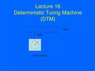
tape head Finite Control Lecture 16 Deterministic Turing Machine (DTM) e p h B a l a The tape has the left end but infinite to the right. It is divided into cells. Each cell contains a symbol in an alphabet Γ . There exists a special symbol B which represents the empty cell. a

Lecture 16 Deterministic Turing Machine (DTM)
E N D
Presentation Transcript
tape head Finite Control Lecture 16Deterministic Turing Machine (DTM)
e p h B a l a The tape has the left end but infinite to the right. It is divided into cells. Each cell contains a symbol in an alphabet Γ. There exists a special symbol B which represents the empty cell.
a • The head scans at a cell on the tape and can read, erase, and write a symbol on the cell. In each move, the head can move to the right cell or to the left cell (or stay in the same cell).
The finite control has finitely many states which form a set Q. For each move, the state is changed according to the evaluation of a transition function δ : Q x Γ → Q x Γ x {R, L}.
b a • δ(q, a) = (p, b, L) means that if the head reads symbol a and the finite control is in the state q, then the next state should be p, the symbol a should be changed to b, and the head moves one cell to the left. q p
a b • δ(q, a) = (p, b, R) means that if the head reads symbol a and the finite control is in the state q, then the next state should be p, the symbol a should be changed to b, and the head moves one cell to the right. q p
There are some special states: an initial state s and an final states h. • Initially, the DTM is in the initial state and the head scans the leftmost cell. The tape holds an input string. s
x • When the DTM is in the final state, the DTM stops. An input string x is accepted by the DTM if the DTM reaches the final state h. • Otherwise, the input string is rejected. h
The DTM can be represented by M = (Q, Σ, Γ, δ, s) where Σ is the alphabet of input symbols. • The set of all strings accepted by a DTM M is denoted by L(M). We also say that the language L(M) is accepted by M.
The transition diagram of a DTM is an alternative way to represent the DTM. • For M = (Q, Σ, Γ, δ, s), the transition diagram of M is a symbol-labeled digraphG=(V, E) satisfying the following: V = Q (s = , h = ) E = { p q | δ(p, a) = (q, b, D)}. a/b,D
1/1,R 0/0,R; 1/1,R 0/0,R 0/0,R B/B,R s p q h 1/1,R M=(Q, Σ, Γ, δ, s) where Q = {s, p, q, h}, Σ = {0, 1}, Г = {0, 1, B}. δ 0 1 B s (p, 0, R) (s, 1, R) - p (q, 0, R) (s, 1, R) - q (q, 0, R) (q, 1, R) (h, B, R) L(M) = (0+1)*00(0+1)*.
Theorem. Every regular set can be accepted by a DTM. Proof. • Every regular set can be accepted a deterministic finite automata (DFA). • Every DFA can be simulated by a DTM.
Review on Regular Set • Regular sets on an alphabet Σis defined recursively as follows (1) The empty set Φ is a regular set. (2) For every symbol a in Σ, {a} is a regular set. (3) If A and B are regular sets, then A ∩ B, A U B, and A* are all regular sets.
Review on DFA tape a b c d e f head finite control
The tape is divided into cells. Each cell contains a symbol in an alphabet Σ. • The head scans at a cell on the tape and can read symbol from the cell. It can also move from left to right, one cell per move.
The finite control has finitely many states which form a set Q. For each move, the state is changed according to the evaluation of a function δ: Q x Σ →Q. If the head reads symbol a and the finite control is in the state q, then the next state is p = δ(q, a).
There are some special states: an initial state s and some final states which form a set F. • The DFA can be represented by M = (Q, Σ, δ, s, F).
Initially, the DFA is in the initial state and the head scans the leftmost cell. The tape holds an input string x. When the head moves off the tape, the DFA stops. An input string is accepted by the DFA if the DFA stops in a final state. Otherwise, the input string is rejected.
Simulate DFA by DTM • Given a DFA M = (Q, Σ, δ, s, F), we can construct a DTM M’ = (Q’, Г, Σ, δ’, s) to simulate M as follows: • Q’ = Q U {h}, Γ = Σ U {B}, • If δ(q, a) = p, then δ’(q, a) = (p, a, R). δ’(q, B) = (h, B, R) for q in F.
1/1,R 0/0,R; 1/1,R 0/0,R 0/0,R B/B,R s p q h 1/1,R L(M) = (0+1)*00(0+1)*. 1 0, 1 0 0 s p q 1
Turing acceptable languages Regular languages
Why DTM can accept more languages than DFA? Because • The head can move in two directions. (No!) • The head can erase. (No!) • The head can erase, write and move in two directions. (Yes!) • What would happen if the head can read, erase and write, but move in one direction?
├ ├
(s, 0110B) ├ (q0, B110B) ├ (q1, B010B) ├ (q1, B010B) ├ (q0, B011B) ├ (h, B0110B)
R {ww | w ε (0+1)*} is Turing-acceptable. (s, B0110B)├ (q, B0110B)├ (q0, B011BB) ├* (q0, B011B) ├ (p0, B011B)├ (ok, BB11B) ├* (ok, B11B) ├ (q, B11B) ├ (q1, B1BB) ├ (q1, B1B) ├ (p1, B1B) ├ (ok, BBB) ├ (q, BBB) ├ (h, BBB) ?? Could we do (ok, BBB) ├ (h, BBB) ?
R L= {ww | w in (0+1)*}
Turing-Computable Functions • A total function f: Σ* → Σ* is Turing-computable if there exists a DTM M such that for every x in Σ*, (s, BxB) ├* (h, Bf(x)B). • A partialf: Ω→ Σ* is Turing-computable if there exists a DTM M such that L(M)=Ω and for every x in Ω, (s, BxB) ├* (h, Bf(x)B).
R The following function f is Turing-computable: f(x) =w, if x = ww ; ↑, otherwise (s, B0110B)├ (q, B0110B)├ (q0, B011BB) ├* (q0, B011B) ├ (p0, B011B)├ (ok, B0’11B) ├* (ok, B0’11B) ├ (q, B0’11B) ├ (q1, B0’1BB) ├ (q1, B0’1B) ├ (p1, B0’1B) ├ (ok, B0’1’B) ├ (q, B0’1’B) ├ (r, B0’1B) ├* (r, B01B) ├ (o, B01B) ├* (o, B01B)├ (k, B01BB) ├ (h, B01B)
R • f(x) = w if x = ww ; ↑, otherwise
Turing-decidable • A language A is Turing-decidable if its characteristic function is Turing-computable. Χ (x) = { 1, if x ε A 0, otherwise A
R • { ww | w ε (0+1)*} is Turing-decidable. (s, B0110B)├ (q, B0110B)├ (q0, B011BB) ├* (q0, B011B) ├ (p0, B011B)├ (ok, B$11B) ├* (ok, B$11B) ├ (q, B$11B) ├ (q1, B$1BB) ├ (q1, B$1B) ├ (p1, B$1B) ├ (ok, B$$B) ├ (q, B$$B) ├ (r, B$BB) ├* (r, BBB) ├ (o, BBB) ├* (h, B1B)
Theorem • A language A is Turing-acceptable iff there exists a total Turing-computable function f such that A = { f(x) | x ε (0+1)*}. • If we look at each natural number as a 0-1 string, then f can be also a total Turing-computable function defined on N, the set of all natural numbers, that is, A = { f(1), f(2), f(3), …} • Therefore, “Turing-acceptable” is also called “recursively enumerable” (r.e.).
Theorem • A language A is Turing-decidable iff A and its complement Ā are Turing-acceptable. Proof. Suppose L(M) = A and L(M’) = Ā. Construct M* to simulate M and M’ simultaneously
Turing-decidable (recursive) Turing-acceptable (r.e.) regular