Turing Machine
Turing Machine. Turing Machines Recursive and Recursively Enumerable Languages. Turing-Machine Theory. The purpose of the theory of Turing machines is to prove that certain specific languages have no algorithm. Start with a language about Turing machines themselves.

Turing Machine
E N D
Presentation Transcript
Turing Machine Turing Machines Recursive and Recursively Enumerable Languages
Turing-Machine Theory • The purpose of the theory of Turing machines is to prove that certain specific languages have no algorithm. • Start with a language about Turing machines themselves. • Reductions are used to prove more common questions undecidable.
Picture of a Turing Machine Action: based on the state and the tape symbol under the head: change state, rewrite the symbol and move the head one square. State . . . . . . A B C A D Infinite tape with squares containing tape symbols chosen from a finite alphabet
Why Turing Machines? • Why not deal with C programs or something like that? • Answer: You can, but it is easier to prove things about TM’s, because they are so simple. • And yet they are as powerful as any computer. • More so, in fact, since they have infinite memory.
Turing-Machine Formalism • A TM is described by: • A finite set of states (Q, typically). • An input alphabet (Σ, typically). • A tape alphabet (Γ, typically; contains Σ). • A transition function (δ, typically). • A start state (q0, in Q, typically). • A blank symbol (B, in Γ- Σ, typically). • All tape except for the input is blank initially. • A set of final states (F ⊆ Q, typically).
Conventions • a, b, … are input symbols. • …, X, Y, Z are tape symbols. • …, w, x, y, z are strings of input symbols. • , ,… are strings of tape symbols.
The Transition Function • Takes two arguments: • A state, in Q. • A tape symbol in Γ. • δ(q, Z) is either undefined or a triple of the form (p, Y, D). • p is a state. • Y is the new tape symbol. • D is a direction, L or R.
Example: Turing Machine • This TM scans its input right, looking for a 1. • If it finds one, it changes it to a 0, goes to final state f, and halts. • If it reaches a blank, it changes it to a 1 and moves left.
Example: Turing Machine – (2) • States = {q (start), f (final)}. • Input symbols = {0, 1}. • Tape symbols = {0, 1, B}. • δ(q, 0) = (q, 0, R). • δ(q, 1) = (f, 0, R). • δ(q, B) = (q, 1, L).
q Simulation of TM δ(q, 0) = (q, 0, R) δ(q, 1) = (f, 0, R) δ(q, B) = (q, 1, L) . . . B B 0 0 B B . . .
q Simulation of TM δ(q, 0) = (q, 0, R) δ(q, 1) = (f, 0, R) δ(q, B) = (q, 1, L) . . . B B 0 0 B B . . .
q Simulation of TM δ(q, 0) = (q, 0, R) δ(q, 1) = (f, 0, R) δ(q, B) = (q, 1, L) . . . B B 0 0 B B . . .
q Simulation of TM δ(q, 0) = (q, 0, R) δ(q, 1) = (f, 0, R) δ(q, B) = (q, 1, L) . . . B B 0 0 1B . . .
q Simulation of TM δ(q, 0) = (q, 0, R) δ(q, 1) = (f, 0, R) δ(q, B) = (q, 1, L) . . . B B 0 0 1B . . .
f Simulation of TM δ(q, 0) = (q, 0, R) δ(q, 1) = (f, 0, R) δ(q, B) = (q, 1, L) No move is possible. The TM halts and accepts. . . . B B 0 0 0B . . .
Instantaneous Descriptions of a Turing Machine • Initially, a TM has a tape consisting of a string of input symbols surrounded by an infinity of blanks in both directions. • The TM is in the start state, and the head is at the leftmost input symbol.
TM ID’s – (2) • An ID is a string q, where includes the tape between the leftmost and rightmost nonblanks. • The state q is immediately to the left of the tape symbol scanned. • If q is at the right end, it is scanning B. • If q is scanning a B at the left end, then consecutive B’s at and to the right of q are part of .
TM ID’s – (3) • As for PDA’s we may use symbols ⊦ and ⊦* to represent “becomes in one move” and “becomes in zero or more moves,” respectively, on ID’s. • Example: The moves of the previous TM are q00⊦0q0⊦00q⊦0q01⊦00q1⊦000f
Formal Definition of Moves • If δ(q, Z) = (p, Y, R), then • qZ⊦Yp • If Z is the blank B, then also q⊦Yp • If δ(q, Z) = (p, Y, L), then • For any X, XqZ⊦pXY • In addition, qZ⊦pBY
Languages of a TM • A TM defines a language by final state, as usual. • L(M) = {w | q0w⊦*I, where I is an ID with a final state}. • Or, a TM can accept a language by halting. • H(M) = {w | q0w⊦*I, and there is no move possible from ID I}.
Equivalence of Accepting and Halting • If L = L(M), then there is a TM M’ such that L = H(M’). • If L = H(M), then there is a TM M” such that L = L(M”).
Proof of 1: Final State -> Halting • Modify M to become M’ as follows: • For each final state of M, remove any moves, so M’ halts in that state. • Avoid having M’ accidentally halt. • Introduce a new state s, which runs to the right forever; that is δ(s, X) = (s, X, R) for all symbols X. • If q is not a final state, and δ(q, X) is undefined, let δ(q, X) = (s, X, R).
Proof of 2: Halting -> Final State • Modify M to become M” as follows: • Introduce a new state f, the only final state of M”. • f has no moves. • If δ(q, X) is undefined for any state q and symbol X, define it by δ(q, X) = (f, X, R).
Recursively Enumerable Languages • We now see that the classes of languages defined by TM’s using final state and halting are the same. • This class of languages is called the recursively enumerable languages. • Why? The term actually predates the Turing machine and refers to another notion of computation of functions.
Recursive Languages • An algorithm is a TM, accepting by final state, that is guaranteed to halt whether or not it accepts. • If L = L(M) for some TM M that is an algorithm, we say L is a recursive language. • Why? Again, don’t ask; it is a term with a history.
Example: Recursive Languages • Every CFL is a recursive language. • Use the CYK algorithm. • Almost anything you can think of is recursive.
More About Turing Machines “Programming Tricks” Restrictions Extensions Closure Properties
Programming Trick: Multiple Tracks • Think of tape symbols as vectors with k components, each chosen from a finite alphabet. • Makes the tape appear to have k tracks. • Let input symbols be blank in all but one track.
Represents input symbol 0 Represents the blank Represents one symbol [X,Y,Z] Picture of Multiple Tracks q 0 X B B Y B B Z B
track 1 track 2 track 1 track 2
Programming Trick: Marking • A common use for an extra track is to mark certain positions. • Almost all tape squares hold B (blank) in this track, but several hold special symbols (marks) that allow the TM to find particular places on the tape.
Unmarked W and Z Marked Y Marking q B X B W Y Z
Programming Trick: Caching in the State • The state can also be a vector. • First component is the “control state.” • Other components hold data from a finite alphabet. • Turing Maching with Storage
Example: Using These Tricks • This TM doesn’t do anything terribly useful; it copies its input w infinitely. • Control states: • q: Mark your position and remember the input symbol seen. • p: Run right, remembering the symbol and looking for a blank. Deposit symbol. • r: Run left, looking for the mark.
Example – (2) • States have the form [x, Y], where x is q, p, or r and Y is 0, 1, or B. • Only p uses 0 and 1. • Tape symbols have the form [U, V]. • U is either X (the “mark”) or B. • V is 0, 1 (the input symbols) or B. • [B, B] is the TM blank; [B, 0] and [B, 1] are the inputs.
The Transition Function • Convention: a and b each stand for “either 0 or 1.” • δ([q,B], [B,a]) = ([p,a], [X,a], R). • In state q, copy the input symbol under the head (i.e., a ) into the state. • Mark the position read. • Go to state p and move right.
Transition Function – (2) • δ([p,a], [B,b]) = ([p,a], [B,b], R). • In state p, search right, looking for a blank symbol (not just B in the mark track). • δ([p,a], [B,B]) = ([r,B], [B,a], L). • When you find a B, replace it by the symbol (a ) carried in the “cache.” • Go to state r and move left.
Transition Function – (3) • δ([r,B], [B,a]) = ([r,B], [B,a], L). • In state r, move left, looking for the mark. • δ([r,B], [X,a]) = ([q,B], [B,a], R). • When the mark is found, go to state q and move right. • But remove the mark from where it was. • q will place a new mark and the cycle repeats.
Semi-infinite Tape • We can assume the TM never moves left from the initial position of the head. • Let this position be 0; positions to the right are 1, 2, … and positions to the left are –1, –2, … • New TM has two tracks. • Top holds positions 0, 1, 2, … • Bottom holds a marker, positions –1, –2, …
0 1 2 3 . . . q * -1 -2 -3 . . . U/L Put * here at the first move You don’t need to do anything, because these are initially B. Simulating Infinite Tape by Semi-infinite Tape State remembers whether simulating upper or lower track. Reverse directions for lower track.
More Restrictions • Two stacks can simulate one tape. • One holds positions to the left of the head; the other holds positions to the right. • In fact, by a clever construction, the two stacks to be counters = only two stack symbols, one of which can only appear at the bottom.
Extensions • More general than the standard TM. • But still only able to define the samelanguages. • Multitape TM. • Nondeterministic TM. • Store for name-value pairs.
Multitape Turing Machines • Allow a TM to have k tapes for any fixed k. • Move of the TM depends on the state and the symbols under the head for each tape. • In one move, the TM can change state, write symbols under each head, and move each head independently.