Tasks 4.1 4.2
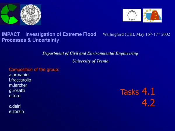
IMPACT Investigation of Extreme Flood Processes & Uncertainty. Wallingford (UK), May 16 th -17 th 2002. Department of Civil and Environmental Engineering University of Trento. Composition of the group: a.armanini l.fraccarollo m.larcher g.rosatti e.toro c.dalrì e.zorzin.

Tasks 4.1 4.2
E N D
Presentation Transcript
IMPACT Investigation of Extreme Flood Processes & Uncertainty Wallingford (UK), May 16th-17th 2002 Department of Civil and Environmental Engineering University of Trento Composition of the group:a.armaninil.fraccarollom.larcherg.rosattie.toroc.dalrìe.zorzin Tasks 4.1 4.2
A Godunov method for the computation of erosional shallow water transients L. Fraccarollo, H. Capart, and Y. Zech submitted to the Int. Journal of Numerical Methods in Fluids, 2002.
Undergoing Advancements • 1D with sections having varying shape and dimensions • inclusions of non-erodible sections at assigned positions • Adaptation processes • Selection processes • Boundary conditions • True two phase flows
A splitting technique is adopted, spanned over two steps for each direction. First step. The numerical integration in the time-space domain concerns the following PDE Second step. The numerical integration in the same domain of the following ODE:
Undergoing Advancements • inclusions of non-erodible sections at assigned positions • Adaptation processes • Selection processes • Boundary conditions • True two phase flows • Rheological model • mesh-cells fitting to boundaries (I.e.:cut-cell methods)
OBLIQUE FRONT DEVIATION ANGLE DEFLECTION ANGLE
belt flume slit 6.0 m uniform granular flow Task 4.2 uniform mud flow Recirculating experimental channel for uniform granular flow
Recirculating experimental channel for uniform granular flow
Recirculating experimental channel for uniform granular flow
Measurement Techniques • Voronoï 2D (Capart et al., 2002) • Voronoï 3D (Spinewine et al., 2002) • PIV (Lorenzi et al., 2002)
Tangential stress local equilibrium Deriving along y and substituting dc/dy we obtain: Second order equation to get velocity profile Local stress relations Normal stress local equilibrium Deriving along y direction:
Experimental installation for mud-flow inflow Feed pipe flume hopper Valve outflow Pneumatic piston (23° max) Pump Forced flux between pump and hopper
Mud-flow (Sarno material) steady condition
Measurement Techniques • Ultrasound doppler velocimeter • Particle tracking • High-frequency radar
Ultrasound Doppler Velocimeter Sampling volume Beam geometry Cardiovascoularsurgery It has been used for medical applications in the 60es; Metallergic industry Food industry Ultrasound beam survey Burst lenght Acoustic field intensity along the transducer Divergence of ultrasonic beam Near field (blind zone) Far field
Working scheme Doppler effect Frequency difference between the sent and the received signal Pulsed doppler ultrasound Shift phase of the received echo Particle velocity
Sound celerity measure geometric field kinematic field Sound celerity determines Micrometer 2MHz probe water 1498 m/s mud 30 % 2100 m/s 2790 m/s mud 40 % Signal Completely absorbed mud 50% Steel plate
Flow direction Z X Y Doppler Angle Doppler angle Ultrasonic Gel Operative procedure 500 kHz probe Side measurements Y is constant Bottom measurements Motion along Z Motion along X Partial ultrasound beam Complete ultrasonic beam
Experiemntal measurements Instrument setting parameters Side measurements 3D velocity profile Mean value over 1000 profiles Concentration variation along the section? Wall reflection effect? Other effects?
Experimentalmeasurements Conclusions about the velocimeter Advantages: - Opaque fluids measurement - Instantaneous geometric-kinematic information Disadvantages: - Distruction of the ultrasonic beam with d> 1.5 mm - Rapid absorption, power increase - High divergence of the sonic field - Invalid data - High Signal Noise Ratio - Sound celerity constant for every fluid