Numerical Optimization

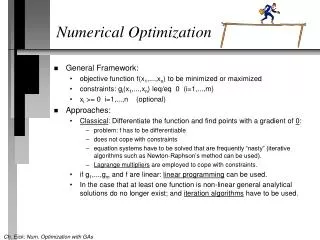
1. Numerical Optimization • General Framework: • objective function f(x1,...,xn) to be minimized or maximized • constraints: gi(x1,...,xn) leq/eq 0 (i=1,...,m) • xi >= 0 i=1,...,n (optional) • Approaches: • Classical: Differentiate the function and find points with a gradient of 0: • problem: f has to be differentiable • does not cope with constraints • equation systems have to be solved that are frequently “nasty” (iterative algorithms such as Newton-Raphson’s method can be used). • Lagrange multipliers are employed to cope with constraints. • if g1,...,gm and f are linear: linear programming can be used. • In the case that at least one function is non-linear general analytical solutions do no longer exist; and iteration algorithms have to be used.

2. Popular Numerical Methods • Newton-Raphson’s Method to solve: f(x)=0 • f(x) is approximated by its tangent at the point (xn, f(xn)) and xn+1 is taken as the abcissa of the point of intersection of the tangent with the x-acis; that is, xn+1 is determined using: f(xn) + (xn+1xn)f’(xn) = 0 • xn+1 = xn + hn with hn = (f(xn) / f’(xn)) • the iterations are broken off when |hn| is less than the largest tolerable error. • The Simplex Method is used to optimize a linear function with a set of linear constraints (linear programming). Quadratic programming [31] optimizes a quadratic function with linear constraints. • Other interation methods (similar to Newton’s method) relying on xv+1= xvvdv where dv is a direction and v denotes the “jump” performed in the particular direction. • Use quadratic/linear approximations of the optimization problem, and solve the optimization problem in the approximated space. • Other popular optimization methods: the penalty trajectory method [220], the sequential quadratic penalty function method, and the SOLVER method [80].

3. Numerical Optimization with GAs • Coding alternatives include: • binary coding • Gray codes • real-valued GAs • Usually lower and upper bounds for variables have to be provided as the part of the optimization problem. Typical operators include: • standard mutation and crossover • non-uniform and boundary mutation • arithmetical , simple, and heuristic crossover • Constraints are a major challenge for function optimization. Ideas to cope with the problem include: • elimination of equations through variable reduction. • values in a solution are dynamic: they are nolonger independent of each other, but rather their contents is constrainted by the contents of other variables of the solution: in some cases a bound for possible changes can be computed (e.g. for convex search spaces (GENOCOP)). • penalty functions. • repair algorithms (GENETIC2)

4. Penalty Function Approach Problem: f(x1,...,xn) has to be maximized with constraints gi(x1,...,xn) leq/eq 0 (i=1,...,m) • define a new function: f’(x1,...,xn)= f(x1,...,xn) + i=1,mwihi (x1,...,xn) with: • For gi(x1,...,xn) = 0: hi(x1,...,xn):= gi(x1,...,xn) • For gi(x1,...,xn) <= 0: hi(x1,...,xn):= IFgi(x1,...,xn) < 0 THEN 0 ELSE gi(x1,...,xn) • Remarks Penalty Function Approach: • needs a lot of fine tuning, especially the selection of weights wi is very critical for the performance of the optimizer. • frequently, the GA gets deceived only exploring the space of illegal solution, especially if penalties are too low; on the other hand, situations of premature convergence can arise when the GA terminates with a local minimum that is surrounded by illegal solutions, so that the GA cannot escape the local minimum, because the penalty for traversing illegal solutions is too high. • a special approach called sequential quadratic penalty function method[9,39] has gained significant popularity.

5. Sequential Quadratic Penalty Function Method • Idea: instead of optimizing the constrainted function f(x), optimize: F(x,r) = f(x) + (1/(2r))(h1(x)2+...+hm(x)2) • It has been shown by Fiacco et al. [189] that the solutions of optimizing the constrainted function f and the solutions of optimizing F are identical for r--0. However, it turned out to be difficult to minimize F in the limit with Newton’s method (see Murray [220]). More recently, Broyden and Attila [39,40] found a more efficient method; GENOCOP II that is discussed in our textbook employs this method.

6. Basic Loop of the SQPF Method 1) Differentiate F(x,r) yielding F’(x,r); 2) Choose a starting vector x0, choose a starting value ro>0; 3) r’:= ro; x’:=x0; REPEAT Solve F’(x,r’)=G(x)=0 for starting vector x’ yielding vector x1; x’:=x1; Decrease r’ by division through >1 UNTIL r’ is sufficiently close to 0; RETURN(x’);

7. Various Numerical Crossover Operators Let p1=(x1,y1) and p2=(x2,y2); crossover operators crossover(p1,p2) include: simple crossover: maxa(x1,y2a+y1 (1-a)); maxa(x2,y1a+y2(1-a)) Whole arithmetical crossover: ap1 + (1-a)p2 with a[0,1] heuristic crossover(Wright[312]): p1 + (p1p2)a with a[0,1] if f(p1)>f(p2) Example: let p1=(1,2), p2=(5,1) be points a convex 2D-space: x2+y2 leq 28 and f(p1)>f(p2) a=1.0 phc=(-3,3) a=0.25 phc’=(0, 2.25) p1=(1,2) psc1=(5,1.7) p2=(5,1) psc2=(1,1) simple crossover yields: (1,1) and (5,sqrt(3)) (25+3=28). arithmetical crossover yields: all points along the line between p1 and p2. heuristic crossover yields: all points along the line between p1 and phc=(-3,3).

8. Another Example (Crossover Operators) Let p1=(0,0,0) and p2=(1,1,1) in an unconstrainted search space: arithmetical crossover produces: (a,a,a) with a[0,1] simple crossover produces: (0,0,1), (0,1,1), (1,0,0), and (1,1,0). heuristic crossover produces: (a,a,a) with a[1,2], if f((1,1,1))>f((0,0,0)) (a,a,a) with a[-1,0], if f((1,1,1))<f((0,0,0)) (1,1,1) (0,0,0)

9. Problems of Optimization with Constraints S legal solutions illegal solutions illegal solutions S S S+ S S legal solutions S:= a solution S+:= the optimal solution

10. A Harder Optimization Problem legal solutions legal solutions illegal solutions illegal solutions legal solutions

11. A Friendly Convex Search Space illegal solutions pu p1 p legal solutions p2 illegal solutions illegal solutions pl Convexity (1) p1 and p2 in S => all points between p1 and p2 are in S (2) p in S => exactly two borderpoints can be found: pu and pl