MA05136 Numerical Optimization
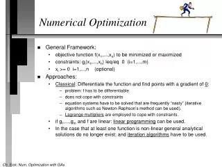
MA05136 Numerical Optimization. 06 Quasi-Newton Methods. Hessian matrix. The Hessian matrix B is needed in computing Newton’s direction p k = − B k −1 f k . What needed is the inverse multiplying a vector. Approximate result maybe good enough in use.

MA05136 Numerical Optimization
E N D
Presentation Transcript
MA05136 Numerical Optimization 06 Quasi-Newton Methods
Hessian matrix • The Hessian matrix B is needed in computing Newton’s direction pk = −Bk−1fk. • What needed is the inverse multiplying a vector. • Approximate result maybe good enough in use. • Quasi-Newton: use gradient vector to approximate Hessian • DFP and BFGS updating formula • SR1 (Symmetric Rank 1 update) method • Broyden class
The secant formula • Suppose we have Hessian Bk at current point xk • Next point is • The model at xk+1 is • Assumeand let and • Then we have the secant formula • Also require Bk+1 to be spd
DFP updating formula • The problem of approximating Bk+1 becomes subject to • With some special norm, the solution is • This is the DFP updating formula • Davidon, Fletcher and Powell
BFGS updating formula • Let . Similar results can be obtained subject to • The solution is • This is the BFGS updating formula • Broyden, Fletcher, Goldfarb, and Shanno
More on BFGS • The initial H0 need be constructed • Finite difference or automatic differentiation (chap 8) • Using identity matrix or • Hessian Bk can be constructed via the Sherman-Morrison-Woodbury formula (rank 2 update) • If Hk is positive definite, Hk+1 is positive definite.
The SR1 method • Desire a symmetric rank 1 update, Bk+1=Bk+vvT, that satisfies the secant constrain: yk=Bk+1sk. • Vector v is parallel to (yk−Bksk). Let v = (yk−Bksk) • Substitute back to the secant constrain • Let zk = yk−Bksk. The SR1 is
More on the SR1 • Let wk = sk− Hkyk. By Sherman-Morrison formula, • If yk= Bksk, Bk+1= Bk. • If ykBksk but (yk−Bksk)Tsk=0, there is no the SR1. • If (yk−Bksk)Tsk 0, the SR1 is numerical instable. • Use Bk+1= Bk. • In practice, the Bk generated by the SR1 satisfies
The Broyden class • The Broyden class is a family of quasi-Newton updating formulas that have the form • k is a scalar function. • It is a linear combination of BFGS and DFP • It is a restricted Broyden class if [0,1]
More on the Broyden class • The SR1 is also belong to the Broyden class with • But may not be belong to the restricted Broyden class. • If k+1 0 and Bk is positive definite, then Bk is positive definite.
Convergence of BFGS • Global convergence For any spdB0 and any x0, if f is twice continuously differentiable and the working set is convex with properly bounded Hessian, then the BFGS converges to the minimizerx* of f. • Convergent rate If f is twice continuously differentiable and 2f is Lipschitz continuous near x*, and then the BFGS converges superlinearly