Download
1 / 51
520 likes | 1.05k Views
Confounding, Matching, and Related Analysis Issues. Kevin Schwartzman MD Lecture 8a June 22, 2005. Confounding, Matching & Related Analysis Issues. Readings Fletcher, chapter 1

E N D
Confounding, Matching, and Related Analysis Issues Kevin Schwartzman MD Lecture 8a June 22, 2005
Confounding, Matching & Related Analysis Issues Readings • Fletcher, chapter 1 • Hennekens and Buring, Epidemiology in Medicine, 1987: Chapter 12, Analysis of Epidemiologic Studies: Evaluating the Role of Confounding [course pack]
Confounding, Matching & Related Analysis Issues - Slide 1 Objectives Students will be able to: 1. Define confounding 2. Explain what must be true of a confounding variable 3. Describe design strategies for control of confounding a. Restriction b. Randomization, including stratified design c. Matching, including different matching schemes
Confounding, Matching & Related Analysis Issues - Slide 2 Objectives 4. Describe analytic strategies for control of confounding a. Stratified analyses b. Standardization c. Calculation of pooled effect estimates: the example of the Mantel-Haenszel odds ratio d. The special case of matched pair case-control studies e. Multivariate analyses 5. Identify advantages and disadvantages of matching 6. Define and identify effect modification
Confounding, Matching & Related Analysis Issues - Slide 3 Confounding • Refers to distortion of the true underlying relationship (or lack thereof) between an exposure and an outcome of interest, because of the influence of a third factor (a “confounder” or a “confounding variable”) • At the design phase, confounding is potential; its true presence or absence is assessed through appropriate data analyses
Confounding, Matching & Related Analysis Issues - Slide 4 Confounding Variables A variable is said to be a confounder if: - it is associated with the exposure of interest - it is an independent risk factor for the outcome of interest - it is not an intermediate along the causal pathway from exposure to outcome Exposure Confounder Outcome
Confounding, Matching & Related Analysis Issues - Slide 6 Case-Control Study
Confounding, Matching & Related Analysis Issues - Slide 7 Smoking as Confounder Smoking was associated with coffee drinking - 400/450 coffee drinkers were smokers, vs 80/230 non-coffee drinkers Smoking is an independent risk factor for lung cancer - here, OR = (300 x 160)/(40 x 180) = 6.7 By separating the group into smokers and non-smokers, and examining the relationship between coffee and lung cancer within each subgroup, confounding by smoking was eliminated
Confounding, Matching & Related Analysis Issues - Slide 8 Smoking as Confounder There was no independent association of coffee drinking with lung cancer (odds ratio within both smoking subgroups or strata was 1) The apparent relationship was due entirely to confounding by smoking Confounding can also reduce, eliminate, exaggerate, or even change the direction of true underlying associations The presence of confounding can be assessed by comparing crude and adjusted effect estimates (some investigators use 10% “rule of thumb”)
Confounding, Matching & Related Analysis Issues - Slide 9 Design Strategies to Control Confounding First of all, any potential confounder must be measured appropriately Simplest strategy (in terms of design) is restriction, to eliminate variation in potential confounder If there is no variation in the potential confounder, it cannot influence the outcome Example: restriction of the lung cancer-coffee study to smokers only However, in this particular case, there could still be residual variation in smoking which could influence outcome
Confounding, Matching & Related Analysis Issues - Slide 10 Randomization Goal is to distribute potential confounders equally between study groups Again, if there is no variation in a potential confounder, it cannot be responsible for differences in outcome Smaller sample sizes may lead to imbalance between groups with respect to potential confounders, simply by chance
Confounding, Matching & Related Analysis Issues - Slide 11 Randomization Stratified randomization (often combined with blocked randomization): promotes equal distribution of treatment groups across strata of variable(s) of interest e.g. gender, age, study centre Number of strata limited by logistical constraints All reports of randomized studies include a table for assessing the adequacy of randomization As soon as analysis is limited to subgroups, the control of confounding disappears e.g. compliance bias (healthy behaviours etc.)
Confounding, Matching & Related Analysis Issues - Slide 12 Matching Matching is an element of observational study design, introduced to help control potential confounders it involves selection of a comparison group that is forced to resemble the index group with respect to the distribution of one or more potential confounders in case-control studies selection of control group (matched to cases with respect to potential confounders) in cohort studies selection of unexposed group (matched to exposed with respect to potential confounders)
Confounding, Matching & Related Analysis Issues - Slide 13 Subjects can be matched for continuous covariates (e.g. age) or categorical covariates (e.g. sex, HIV serology, etc.) Matching may be done at the level of the individual or of the group In a case-control study, individual matching means that each case is separately matched to one or more control(s) according to the matching factor(s) Matching or variable ratio may be fixed (e.g. 1 case:1 control, 1:2, etc.)
Confounding, Matching & Related Analysis Issues - Slide 14 • We will primarily discuss matching in case-control studies • For categorical covariates, individual matching means that for each case, the control subject(s) is/are drawn from the same category, e.g. male controls for male subjects • Continuous covariates may also be “categorized”, e.g. age divided into categorical ranges: 20-39, 40-59, 60-79, etc.
Confounding, Matching & Related Analysis Issues - Slide 15 Continuous variables may be matched by a) Caliper matching: a rule by which values are considered sufficiently close Matching done on sex plus age within 3 years Potential controls: men aged 28, 35, 39, 49, 57 women aged 31, 34, 43 Case 1: 31 y.o. male matched to 28 y.o. male Case 2: 38 y.o. female no match found case discarded or additional controls identified
Confounding, Matching & Related Analysis Issues - Slide 16 Continuous variables may be matched by b) Nearest available matching - controls are selected based on the closest value of the matching factor In above example, the match for the 38 y.o. female case would be a 34 y.o. female control Advantage: less restrictive, more efficient Disadvantage: Subjects may be less well matched if the distribution of the matching variable is quite different between cases and controls
Confounding, Matching & Related Analysis Issues - Slide 17 Example: cases of a disease which affects primarily elderly persons Controls drawn from the general population with matching based on nearest age may be considerably younger, on average, depending on the number of potential controls identified. - the same may occur when continuous variables are categorized into wide ranges - the impact of the study will depend on the nature of the relationship between the matching factor, the exposure, and the outcome of interest
Confounding, Matching & Related Analysis Issues - Slide 18 Group level matching Cases are stratified according to the matching factor, and then controls are selected to match the grouping of cases a) Stratified sampling: The levels of the covariate in which sampling occurs are defined. Then preset numbers of cases and controls are drawn from each stratum, with a consistent matching ratio
Confounding, Matching & Related Analysis Issues - Slide 19 Example of stratified sampling: Case-control study examining coffee intake and lung cancer
Confounding, Matching & Related Analysis Issues - Slide 20 b) Frequency matching There is also a constant proportion of controls to cases, but the distribution of cases is not fixed according to the matching factor. However, controls are forced to have the same distribution of the matching factor as do the cases. The distribution of the matching factors is therefore representative of that among the population that gave rise to cases.
Confounding, Matching & Related Analysis Issues - Slide 21 Example of frequency matching: Coffee intake and lung cancer - here the number of cases in each smoking stratum reflects the distribution of smoking behaviour among lung cancer cases - the matching ratio is 2 controls per case throughout
Confounding, Matching & Related Analysis Issues - Slide 22 Analysis of case-control studies with matching: - Always requires stratification by the matching factor (or the multivariate equivalent - conditional logistic regression). - The crude odds ratio will be biased toward the null value. - This is because matching forces the cases and controls to be more alike with respect to the exposure of interest than would ordinarily be the case.
Confounding, Matching & Related Analysis Issues - Slide 23 Hypothetical example: Obesity Yes No Total Smokers Heart disease 480 20 | 500 No heart disease 420 80 | 500 _________________________________ Total 900 100 | 1000 _________________________________ OR = 4.6 Obesity Yes No Total Non-smokers Heart disease 8 42 | 50 No heart disease 2 48 | 50 _________________________________ Totals 10 90 | 100 _________________________________ OR = 4.6
Confounding, Matching & Related Analysis Issues - Slide 24 Crude analysis of same data Obesity Yes No Total Heart disease 488 62 | 550 No heart disease 422 128 | 550 ____________________ Totals 910 190 | 1100 OR crude = 2.4 Despite matching, the underlying association between smoking (confounder) and obesity (exposure) remains: smokers were much more likely than non-smokers to be obese. However, matching on smoking behaviour made cases and controls more similar with respect to obesity, thereby leading to underestimation of the odds ratio. Stratified analysis corrects this problem.
Confounding, Matching & Related Analysis Issues - Slide 25 Matching in cohort studies - does not lead to inappropriate crude risk/rate ratio estimates e.g. cohort study of obesity and heart disease Obesity Yes No Total Smokers Heart disease 460 100 No heart disease 540 900 _______________________________________ Total 1000 1000 2000 _______________________________________ RR = 4.6 Obesity Yes No Total Non-smokers Heart disease 46 10 No heart disease 954 990 _______________________________________ Total 1000 1000 2000 _______________________________________ RR = 4.6
Confounding, Matching & Related Analysis Issues - Slide 26 Crude analysis Coffee Yes No Totals Smokers Lung cancer 506 110 | 616 No cancer 1494 1890 | 3384 ___________________________________ Totals 2000 2000 | 4000 RR = 4.6 Here the crude RR is the same as within the individual strata. This is because matching eliminates the association between smoking (confounder) and coffee drinking (the exposure studied).
Confounding, Matching & Related Analysis Issues - Slide 27 Stratified Analysis If effect estimates are identical across strata, then it is easy to report a single summary estimate (e.g. odds ratio) More often, they are not precisely identical, which may reflect random error/imprecision (e.g. small strata), residual confounding, or truly different effects (effect modification) Effect modification will be described separately
Confounding, Matching & Related Analysis Issues - Slide 28 Combining Effects from Strata • Can take some type of weighted average • One approach is to use weights which reflect the distribution of the stratification variable in the population of interest • For example, age-specific risk ratios could be combined using a weighted average that accounts for the age distribution of the general population • This is an example of standardization: the effect is adjusted to reflect a standard age distribution • This does not assume that the effects are homogeneous • The most heavily weighted strata may not have much information
Confounding, Matching & Related Analysis Issues - Slide 29 Mantel-Haenszel Odds Ratio • An odds ratio that reflects pooling of effects across strata, to summarize the overall association between exposure and outcome, while adjusting for the effect of the confounder of concern • Pooling assumes that the effect is homogeneous, and variation reflects random error • Is a weighted average of odds ratio estimates across strata • Weights reflect quantity of information in each stratum, expressed as bc/T where b and c are exposed controls and unexposed cases within the stratum, and T is total subjects within the stratum • Note this differs from standardization using “external” weights
Confounding, Matching & Related Analysis Issues - Slide 30 Mantel-Haenszel Odds Ratio OR MH = Σ[(bc/T) x ad/bc] = Σ(ad/T) __________________ _________ Σ(bc/T) Σ(bc/T) For the case-control study of obesity and heart disease, this would be: (480 x 80)/1000 + (8 x 48)/100 __________________________ (20 x 420)/1000 + (42 x 2)/100 = (38.4 + 3.84)/(8.4 + 0.84) = 4.6
Confounding, Matching & Related Analysis Issues - Slide 31 Analysis of matched pair data in case control studies • can be thought of as a special case of stratified analysis • each matched pair constitutes a single stratum with 2 subjects • only informative strata are those where exposure status of case and control are discordant
Confounding, Matching & Related Analysis Issues - Slide 32 Recall Mantel-Haenszel OR estimates OR MH = (ad/T) _______ (bc/T) Concordant strata: E + E - D + 1 0 D - 1 0 or E + E - D + 0 1 D - 0 1 ad = 0, bc = 0
Confounding, Matching & Related Analysis Issues - Slide 33 The pairs can be grouped as follows: Case Control Exposed Unexposed Exposed r s Unexposed t u Then OR MH = t/s i.e. N(case exposed, control unexposed) _____________________________ N(case unexposed, control exposed) where N refers to number of pairs
Confounding, Matching & Related Analysis Issues - Slide 34 Example: Marrie et al conducted a study evaluating the relationship between certain infections (the exposure) and the subsequent development of multiple sclerosis (the outcome). Data was taken from a general practice database. Cases and controls were matched on age ( 2 years), sex, physician practice, and date seen. Imagine a 1:1 design (in fact it was 1:4, on average).
Confounding, Matching & Related Analysis Issues - Slide 35 Hypothetical data MS (cases) No MS (controls) Infection No infection Infection 30 5 No infection 20 170 OR = 20/5 = 4
Confounding, Matching & Related Analysis Issues - Slide 36 Suppose the key confounder is physician practice - the physicians most likely to see and diagnose infections may also be those most likely to pursue and establish the diagnosis of multiple sclerosis Unmatched analysis MS No MS Infection 50 35 No infection 175 190 Crude OR = (190x50) / (175x35) = 1.6 As before, the unstratified analysis yields an OR estimate biased toward the null. As before, this is because the matching forces the controls to “resemble” the cases with respect to the distribution of exposure in the crude analysis.
Confounding, Matching & Related Analysis Issues - Slide 37 Multivariate Analysis Has become the standard approach for identifying and accounting for confounding Complex process: computer essentially solves multiple equations to identify “best guess” effect estimate while holding other covariates constant, e.g. effect of obesity while holding smoking behaviour, sex, diabetes constant Mathematically breaks the data down into numerous strata Examples: logistic regression for binary outcome data (very frequent), Cox proportional hazards modelling for incidence data, Poisson model for count data
Confounding, Matching & Related Analysis Issues - Slide 38 Rationale for Matching • Matching can be considered a form of partial restriction: the controls are restricted so as to resemble the cases with respect to some factor(s). • The main purpose of matching is to improve statistical efficiency (precision). • In principle, stratified analysis alone (including multivariate techniques) should be sufficient to deal with the confounder in question. • However, matching may be needed to ensure that all strata are sufficiently informative.
Confounding, Matching & Related Analysis Issues - Slide 39 Example: An investigator wishes to investigate a possible association between use of calcium channel blockers (drugs used for blood pressure and heart disease) and Alzheimer’s disease. Age is obviously a key confounder: increasing age is associated with use of the drugs in question and with the onset of Alzheimer’s disease Unmatched controls drawn from the general population will be younger and hence less likely to be using calcium channel blockers, leading the crude analysis to overestimate any potential association
Confounding, Matching & Related Analysis Issues - Slide 40 • This can be handled through stratified analysis by age (e.g. various age categories) • If unmatched general population controls are used, there may be few controls in the oldest age strata, leading to imprecise OR estimates in those strata (wide confidence intervals) • Matching ensures sufficient numbers of subjects for each level of the matching variable(s) - in this case, age • Matched cohort studies are also more efficiently analyzed using stratification by the matching factor(s)
Confounding, Matching & Related Analysis Issues - Slide 41 Advantages of matching 1. Promotes efficiency, as discussed above. Studies are most efficient when the the ratio of index to referent subjects (e.g. cases:controls) is constant across the different strata of a confounder. 2. Very useful in situations where the confounder is difficult to quantify or control, making stratification impossible. Classic example: using sibling controls.
Confounding, Matching & Related Analysis Issues - Slide 42 Disadvantages of matching 1. Practical - may be cumbersome, expensive, time consuming. Depending on the circumstances, index subjects may be dropped if no matching referent subjects are found loss of data. Also very onerous when many matching factors are used. 2. The effect of the matching factor on the outcome of interest cannot be evaluated. 3. Potential for overmatching.
Confounding, Matching & Related Analysis Issues - Slide 43 Overmatching Refers in general to situations where matching interferes with the logistics, statistical efficiency, or scientific validity of a study. 1. Overmatching as a cause of logistical inefficiency matching on many factors, or on factors that are difficult to match, adds to the expense and difficulty of study conduct difficulty with matching may lead to loss of cases as well as of potential controls (in case-control studies)
Confounding, Matching & Related Analysis Issues - Slide 44 2. Overmatching as a cause of reduced statistical efficiency occurs when matching factor is not a true confounder, e.g. associated with exposure but not with outcome simplest example is with matched pair case-control design if cases and controls made more similar with respect to exposure frequency, then there will be many uninformative pairs these do not contribute to the odds ratio estimate and are essentially “ wasted” conversely with fewer discordant pairs, the precision of the odds ratio estimate is reduced the same holds true for other matching ratios
Confounding, Matching & Related Analysis Issues - Slide 45 • With weak confounders (e.g. limited effect on outcome) the loss of statistical efficiency may outweigh any apparent benefits of matching • Recall that stratified analysis and multivariate techniques will still account for potential confounders in the absence of matching
Confounding, Matching & Related Analysis Issues - Slide 46 3. Overmatching as a cause of biased effect estimates Occurs when matching factor is: a) produced by exposure and related to disease (e.g. an intermediate in pathway) or b) produced by disease and related to exposure
Confounding, Matching & Related Analysis Issues - Slide 47 Effect Modification • Effect modification refers to the situation where the biologic effect of exposure on outcome differs according to some additional factor, e.g. different influence of smoking on development of COPD in men and women • Also known as interaction • In stratified analysis, will see different exposure-outcome relationships within different strata, e.g. different odds ratios, rate ratios, etc.
Confounding, Matching & Related Analysis Issues - Slide 48 • In the absence of confounding, the overall effect estimate will simply be an average of the stratum-specific estimates, weighted by the size of the strata e.g. males and females • Effect modification is NOT the same as confounding - It refers to biologic variation in an effect, not artefactual distortion of results because of inadequate design or analysis • Effect modification should be noted and reported, rather than “controlled” through design and analysis strategies • Effect modification is relevant to randomized trials as well as observational studies