Download
1 / 39
400 likes | 584 Views
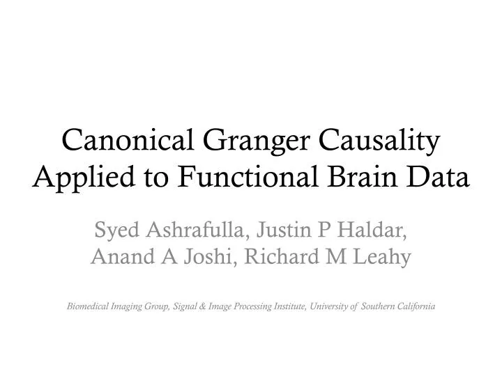
Canonical Granger Causality Applied to Functional Brain Data. Syed Ashrafulla, Justin P Haldar , Anand A Joshi, Richard M Leahy. Biomedical Imaging Group, Signal & Image Processing Institute, University of Southern California.

E N D
Canonical Granger CausalityApplied to Functional Brain Data Syed Ashrafulla, Justin P Haldar, Anand A Joshi, Richard M Leahy • Biomedical Imaging Group, Signal & Image Processing Institute, University of Southern California
We want to determine the dynamics of regions of interest in the brain. Non-invasively Invasively Bressler 1993, Nature www.elekta.sg www.sciencephoto.com Cleveland Clinic
How do we measure information flow between signal generators in the brain? Undirected • Correlation • Coherence ... ... x1[n-1] x2[n-1] x1[n] x2[n]
How do we measure information flow between signal generators in the brain? Undirected Directed Granger causality Solved by autoregression • Correlation • Coherence ... ... ... ... x1[n-1] x2[n-1] x1[n-1] x2[n-1] x1[n] Granger 1969, Econometrica x1[n] x2[n] Sims 1972, Am Econ Rev
Timeseries recorded on the cortex can be segregated into regions of interest.
Timeseries recorded on the cortex can be segregated into regions of interest.
Timeseries recorded on the cortex can be segregated into regions of interest.
Timeseries recorded on the cortex can be segregated into regions of interest. Somatosensory/Motor Visual (Occipital)
Bivariate measures do not summarize relationships between regions of interest.
Bivariate measures do not summarize relationships between regions of interest.
Bivariate measures do not summarize relationships between regions of interest.
Bivariate measures do not summarize relationships between regions of interest.
Bivariate measures do not summarize relationships between regions of interest.
Bivariate measures do not summarize relationships between regions of interest.
We can summarize inter-regional relationships and regional topographies.
We can summarize inter-regional relationships and regional topographies.
We can look at total causality or causality between intra-region projections. • σ(A|B) = error in predicting A from B Bivariate Granger causality y1[n] Geweke 1982, J Amer Stat Assoc Multivariate Granger causality y2[n] Barrett 2010, Phys Rev E Canonical Granger causality Ashrafulla 2012, ISBI
We can look at total causality or causality between intra-region projections. • σ(A|B) = error in predicting A from B Bivariate Granger causality y1[n] Geweke 1982, J Amer Stat Assoc Multivariate Granger causality y2[n] Barrett 2010, Phys Rev E Canonical Granger causality Ashrafulla 2012, ISBI
CGC is more robust and more informative than multivariate GC. Robustness • Fewer degrees of freedom • Let y1 have dimension A and y2 have dimension B • M21 requires autoregression in A+B dimensions • # of parameters = (A+B)2P • R21 requires autoregression in 2 dimensions • # of parameters = 4P + A + B • Stable for shorter timeseries • Resistant to low-rank • M21 requires rank A+B covariances • R21 only requires rank 2 in covariances • Resistant to low-rank cross-covariances
CGC is more robust and more informative than multivariate GC. Robustness Extra information Topographies M21 does not say which channels are important R21 has optimal weights implying estimated topography Weights can determine sub-regional locations of signals • Fewer degrees of freedom • Let y1 have dimension A and y2 have dimension B • M21 requires autoregression in A+B dimensions • # of parameters = (A+B)2P • R21 requires autoregression in 2 dimensions • # of parameters = 4P + A + B • Stable for shorter timeseries • Resistant to low-rank • M21 requires rank A+B covariances • R21 only requires rank 2 in covariances • Resistant to low-rank cross-covariances
Conforming conjugate gradient descent to the constraints speeds up optimization. Gradient Nonlinear Conjugate Gradient Descent Modified Gradient “Line Search” = Geodesic Search
Conforming conjugate gradient descent to the constraints speeds up optimization. Gradient Nonlinear Conjugate Gradient Descent Modified Gradient “Line Search” = Geodesic Search
Conforming conjugate gradient descent to the constraints speeds up optimization. Gradient Nonlinear Conjugate Gradient Descent Modified Gradient “Line Search” = Geodesic Search
Conforming conjugate gradient descent to the constraints speeds up optimization. Gradient Nonlinear Conjugate Gradient Descent Modified Gradient “Line Search” = Geodesic Search
Conforming conjugate gradient descent to the constraints speeds up optimization. Gradient Nonlinear Conjugate Gradient Descent Modified Gradient “Line Search” = Geodesic Search
Conforming conjugate gradient descent to the constraints speeds up optimization. Gradient Nonlinear Conjugate Gradient Descent Modified Gradient “Line Search” = Geodesic Search
Conforming conjugate gradient descent to the constraints speeds up optimization. Gradient Nonlinear Conjugate Gradient Descent Modified Gradient “Line Search” = Geodesic Search
CGC can find direction of flow for shorter timeseries. 5000 samples Canonical GC Bivariate GC: x1 x2 Multivariate GC Bivariate GC: x1 x2
CGC can find direction of flow for shorter timeseries. 5000 samples True Positives: 98.5% Canonical GC Bivariate GC: x1 x2 True Positives: 97.8% Multivariate GC Bivariate GC: x1 x2
CGC can find direction of flow for shorter timeseries. 5000 samples 200 samples True Positives: 98.5% Canonical GC Canonical GC Bivariate GC: x1 x2 Bivariate GC: x1 x2 True Positives: 97.8% Multivariate GC Multivariate GC Bivariate GC: x1 x2 Bivariate GC: x1 x2
CGC can find direction of flow for shorter timeseries. 5000 samples 200 samples True Positives: 98.5% True Positives: 84.5% Canonical GC Canonical GC Bivariate GC: x1 x2 Bivariate GC: x1 x2 True Positives: 97.8% True Positives: 47.6% Multivariate GC Multivariate GC Bivariate GC: x1 x2 Bivariate GC: x1 x2
How does the macaque process visual stimuli in a visuomotor task? • Stimulus: push lever down • 2 conditions: • GO: release lever upon certain visual stimulus • NoGo: keep lever down upon other stimulus • Record local field potentials on macaque cortex
How does the macaque process visual stimuli in a visuomotor task? S3 • Stimulus: push lever down • 2 conditions: • GO: release lever upon certain visual stimulus • NoGo: keep lever down upon other stimulus • Record local field potentials on macaque cortex • S2 • S1 P1 • P2 • IT
Macaques send information from striate to prestriate before deciding on action. Bivariate (spectral) causality
Macaques send information from striate to prestriate before deciding on action. Canonical (spectral) causality Bivariate (spectral) causality
Macaques send information from striate to prestriate before deciding on action. Canonical (spectral) causality with weights P1 S3 • P2 • S2 • IT • S1 Bivariate (spectral) causality
Conclusions • CGC summarizes regional connectivity. • Requires regions known a priori • Regions make signals, not direct sensor locations. • CGC is robust to the number of samples. • Short timeseries • Can use for dynamic connectivity studies • Low-rank signal space • CGC finds topographies within regions. • Weights tell which areas within region contribute • Can find that channels do not participate on own but rather in group.
Thank you! This work was funded under the NIBIB T32EB00438 Bioinformatics Training Program and NIH grants R01EB009048 and R01 5R01EB000473.