Exponential and Logarithmic Functions

1. Exponential and Logarithmic Functions Module 8 Lecture 1

2. Topic 1: The Exponential Function

3. dy = = Solve xy , y ( 0 ) 3 dx • We have seen the exponential function before … In Module 6, Lecture 2 … verifying solutions to DE’s: Show is a solution of the differential equation … solving DE’s:

4. and we have already seen an application with an exponential solution to a DE … Modelling the growth rate of bacteria Note the characteristic upward curve of an exponential solution Modelling with DE’s is so important (widespread), let’s run through a couple more of these problems (they both happen to have an exponential solution)

5. Example A population is growing at a rate of 1.3 times the number present each minute. If there were originally 80 individuals present, how many would be present after 100 minutes.

6. Example A population is growing at a rate of 1.3 times the number present each minute. If there were originally 80 individuals present, how many would be present after 100 minutes. Find N(100)

7. Raise each side as a power of e Note: Drop | | as everything > 0 Find N(100) 0. separate the variables to different sides Note: We are assuming N is continuous 1. Integrate 2. Make N the subject

8. = Use initial condition N ( 0 ) 80 c = where A e Find N(100) 3. Rework the constant 4. Evaluate the constant 5. Answer the question

9. Example A 10kg block of ice is melting in an environment in which the temperature is increasing. The rate of loss of mass, per second, is proportional to 20 minus the weight remaining. After 60 seconds the block weighs 9.5 kg. What is the mass of the block after 120 seconds? Notice that there will be two constants to evaluate, one from the proportionality and one from the integration.

10. Raise each side as a power of e Note: Drop | | as everything M < 20 Find M(120) 0. separate the variables to different sides 1. Integrate 2. Make N the subject The c is now -c

11. c = where A e Find M(120) 3. Rework the constant of integration 4. Evaluate the constants(2 constants need 2 conditions) Use initial condition M(0) = 10 Use condition M(60) = 9.5 Solve for k

12. Find M(120) 5. Answer the question

13. Class Exercise The population, P, of insects in a given region changes according to a fixed birth rate of a insects born per 100 insects in the population. The population triples every two weeks. The current population is 500 insects. How does the population evolve over time? State this problem as a differential equation and solve it.

14. Exponential (and logarithmic) functions have many applications in engineering Applications • Typically used in problems involving growth or decay: • Population modelling • Models of vibrations or earthquakes • Heat transfer • Behaviour of electrical signals • Finance In this module, we will explore the exponential (and logarithm) and its relation to DE’s in more depth

15. Imagine that you just won $400,000 in Lotto. Do you spend the money right away and then spend the rest of your life working … or devise a plan to retire young? Who wants to be a millionaire? • If you invest the money at a rate of interest = r • then after a year you have: • After two years you have:

16. Bank interest rates right now are about 7% so if you invest the money for 10 years at 7% you would have: • If after the 10 years you kept the $786,860 invested at 7% but used the interest as income you would have an income of $55,080 every year.

17. What has financial maths got to do with the exponential function ? Somebody, at least 400 years ago, first came across the number e = 2.718281828459045235 … when working out compound interest We will see where it comes from in the following, where we look at different types of “compound interest” formulae used by lenders

18. A Credit Card … Suppose you have a credit card overdraft of $10,000. The bank adds interest daily at a rate 0.05%. The amount you owe after d days is After 1 day you owe After 1 year you owe … an “effective annual interest rate” of about 20%

19. More generally, if the overdraft is $A and the interest is compounded daily at a rate r%, the amount you owe after d days is This formula is in terms of days d. Banks more usually give interest information in terms of years y … Interest compounded daily at rate r

20. Also, the banks will usually give you the so-called “annual rate” R = 365r, and the formula used is Interest compounded daily at annual rate R Now … if the interest is compounded not daily but, more generally, k times per year, we have Interest compounded k times per year at annual rate R

21. Example You have a credit card overdraft of $10,000 compounded weekly at an annual rate of 20%. Then the overdraft after 6 months is After a year it is or

22. Re-write the interest formula in the form Interest compounded k times per year at annual rate R What happens if the bank offers “continuous compounding”? This means that it compounds non-stop: an “infinite” number of times a year. So what happens when k gets larger and larger?

23. Interest compounded k times per year at annual rate R let us see what happens to the term inside the brackets here as k gets larger and larger e

24. So we finally have the formula Interest compounded continuously at annual rate R The number e next appeared in what seemed a completely different problem …

25. x x = = Here are the graphs of y 2 and y 3 What function is its own derivative ? They both go through the point (0,1) since anything to the power of 0 is 1

26. Next examine the derivatives of these functions, i.e. the “derived functions” As h gets smaller and smaller we get more accuracy for these derivatives

27. h h - - ( 2 1 ) ( 3 1 ) h h Let h 0.1 0.71773 1.16123 0.01 0.69556 1.10467 0.0001 0.69317 1.09867 0.00001 0.69315 1.09862 0.000001 0.69315 1.09861 The table indicates these terms approach constants. Later we will see these constants are ln2 and ln3

28. This is what we have … It looks like there is a function between these two for which

29. Define e to be that number (between 2 and 3) with i.e. ex differentiates to itself

30. The Exponential Function i.e. the function that differentiates to itself • The solution to this DE is written in the form • y = ex • Sometimes this is written as y = exp(x) • e = 2.718282…..

31. The Exponential Function… what you need to know Apart from the modelling problems we saw before, nothing

32. Topic 2: The Logarithmic Function

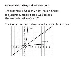
33. The Logarithmic Function - Preliminaries Consider the graph of y=2x shown below. You can read off values from the graph … for example when y=8 you have x=3, since 8=23. Similarly y=24 gives x=4.6, since 24=24.6. In these expressions the number we are taking powers of is called the base. In this case the base is 2. 8 3

34. Think of a log as asking the question: “What power of my base is this number?” so becomes what power of 2 is 1 ? what power of 2 is 8 ? what power of 2 is 24 ?

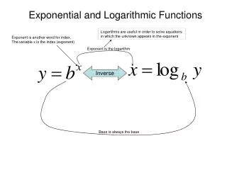
35. The (Natural) Logarithmic Function Consider now the exponential function y = ex We find that, for example The base is now e and the logarithm is Because of the special importance of this particular logarithm, we drop the subscript and use the symbol ln, and call it the natural logarithm …

36. Here is a plot of both the exponential function and the natural logarithm They are inverses of each other: each can be obtained from the other by a reflection in the (dotted) line y = x Properties of ln (and of logs in general) 1. lnx is only defined for x > 0 3. ln1 = 0

37. Is the inverse of the exponential function In summary … the (natural) logarithmic function Remember the | |

38. We want to take the derivative of powers and logs. First, recall the derivation of the derivative of lnx raise both sides as power of e implicit differentiation replace ey by x

39. Differential of ax Strategy: We know how to differentiate ln, so take ln of both sides and differentiate take ln of both sides implicit differentiation Replace y by ax

40. Differential of logax Strategy: We know how to differentiate ln, so write expression as a power of a and then take ln raise both sides as power of a take ln of both sides differentiate both sides

41. General Rule: ax and logax differentiate like ex and lnx with an extra factor of lna

42. Thus, in terms of our initial slides

43. The Logarithmic Function… what you need to know Derive the formulae:

44. Topic 3: Modelling Data with the Exponential and Logarithmic Function

45. Modelling After plotting the points from an experimental “data set” we can get some idea of what function may be used to model the data set. • If it looks like the data is well approximated by exponential functions: plot lnN against t • If it looks like the data is well approximated by power functions: plot lnN against lnt A graphics calculator is very useful for this.

46. Exponential Curve Model Suppose we have the data plotted below: N versus t. It has the “decay” profile of an exponential curve. So let’s assume an exponential model, N=Aekt.

47. The N vs t plot is not a very useful format for determining the unknown coefficients in the N=Aektmodel (A and k). • What if we plotted ln(N) vs t?

48. This plot looks like a straight line – and here’s why: if we take the (natural) log of both sides of our model equation we get

49. We can now read the constants off the lnN versus t plot slope = k ln(N)=ln(A) at t = 0

50. Power Law Model Here is a plot of some data, y versus x. If we don’t get a good fit with the exponential curve model, we can try a power law model y=Axn. Let’s do that here.