Download
1 / 53
660 likes | 1.41k Views
5. Exponential and Logarithmic Functions. Case Study. 5.1 Rational Indices. 5.2 Logarithmic Functions. 5.3 Using Logarithms to Solve Equations. 5.4 Graphs of Exponential and Logarithmic Functions. 5.5 Applications of Logarithms. Chapter Summary.

E N D
5 Exponential and Logarithmic Functions Case Study 5.1 Rational Indices 5.2 Logarithmic Functions 5.3 Using Logarithms to Solve Equations 5.4 GraphsofExponentialandLogarithmicFunctions 5.5 Applications of Logarithms Chapter Summary
The growth rate of bacteria can be expressed by an exponential function. We can use it to find the number of bacteria. How can we find the number of bacteria after a certain period of time? Case Study Although it is not easy to see bacteria with our naked eyes, bacteria do exist almost everywhere. Most bacteria reproduce by cell division, that is, one bacterium can divide and become 2, 2 become 4, and so on. However, each species reproduces itself at different rates due to different humidities and temperatures.
5.1 Rational Indices In general, for a positive integer n, if xny, then x is an nth root of y and we use the radical to denote an nth root of y. Positive nth root: ; Negative nth root: then is not a real number. is usually written as . Examples: then 0 (for 0) and 0 (for y 0). A. Radicals We learnt that if x2y, for y 0, then x is a square root of y. If x3y, then x is a cube root of y. If x4y, then x is a fourth root of y. Remarks: If n is an even number and y 0, then y has one positive nth root and one negative nth root. If n is an even number and y 0, If n is an odd number,
5.1 Rational Indices Try to find the meaning of and : Since Take nth root on both sides, we have . Then consider and Hence we have . B. Rational Indices In junior forms, we learnt the laws of indices for integral indices. Recall that (am)namn, where m and n are integers. y
5.1 Rational Indices 1. 2. where m, n are integers and n 0. The fraction is in its simplest form and n is odd. B. Rational Indices Therefore, for y 0, we define rational indices as follows: Remarks: In the above definition, y is required to be positive. However, the definition is still valid for y 0 under the following situation: For example:
5.1 Rational Indices Simplify , where b 0 and express the answer with a positive index. First express the radical with a rational index. Then use (bm)nbmn to simplify the expression. B. Rational Indices Example 5.1T Solution:
5.1 Rational Indices Evaluate . Change the mixed number into an improper fraction first. B. Rational Indices Example 5.2T Solution:
5.1 Rational Indices Simplify . Change the numbers to the same base before applying the laws of indices. B. Rational Indices Example 5.3T Solution:
5.1 Rational Indices n C. Using a Calculator to Find ym The following is the key-in sequence of finding : 5 32 Since , we can also press the following keys in sequence: 32 2 5 Remarks: If n is an even number and ym 0, then ym has two nth real roots, i.e., . However, the calculator will only display .
5.1 Rational Indices For the equation b, where b is a non-zero constant, p and q are integers with q 0, we can take the power of on both sides and solve the equation: D. Using the Law of Indices to Solve Equations
5.1 Rational Indices If , find x. Change the equation into the form first. D. Using the Law of Indices to Solve Equations Example 5.4T Solution:
5.1 Rational Indices Take out the common factor 22x first. x D. Using the Law of Indices to Solve Equations Example 5.5T Solve 22x 1 22x 8. Solution: 22x1 22x 8 2(22x) 22x 8 22x(2 1) 8 22x 8 22x 23 2x 3
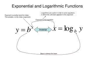
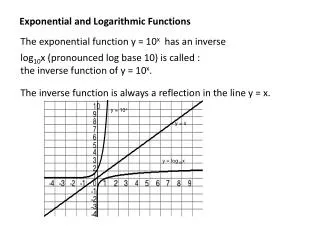
In the calculator, the button log also stands for the common logarithm. 5.2 Logarithmic Functions A. Introduction to Common Logarithm If a number y can be expressed in the form ax, where a 0 and a 1,then x is called the logarithm of the number y to the base a. It is denoted by x logay. If yax, then logay x, where a 0 and a 1. Notes: If y 0, then logay is undefined. Thus the domain of the logarithmic function logay is the set of all positive real numbers of y. When a 10 (base 10), we write log y for log10y. This is called the common logarithm. If y 10n, then log y n. ∴ log 10n n for any real number n.
∵ 102 ∴ log 2 ∵ 101 ∴ log 1 5.2 Logarithmic Functions A. Introduction to Common Logarithm By the definition of logarithm and the laws of indices, we can obtain the following results directly: ∵ 1 100 ∴ log 1 0 ∵ 10 101 ∴ log 10 1 ∵ 100 102 ∴ log 100 2 ∵ 1000 103 ∴ log 1000 3 Values other than powers of 10 can be found by using a calculator. For example: log 34 1.5315 (cor. to 4 d. p.) Given log x1.2. ∴ x 101.2 0.0631 (cor. to 3 sig. fig.)
For M, N 0, 1. log (MN) log M log N 2. log log M log N 3. log Mn n log M Take common logarithm on both sides. In general, 1. log M log N log (MN); 2. ; 3. (log M)n log Mn. Consider ∴ log a b 5.2 Logarithmic Functions B. Basic Properties of Common Logarithm The function f(x) log x, for x 0 is called a logarithmic function. There are 3 important properties of logarithmic functions: Let M 10a and N 10b. Then log M a and log N b. Consider MN 10a 10b 10a b ∴ log (MN) a b log M log N 10a b Consider Mn (10a)n 10na ∴ log Mn na n log M log M log N
Evaluate the following expressions. (a) log 5 log (b) (a) ∴ 5.2 Logarithmic Functions B. Basic Properties of Common Logarithm Example 5.6T Solution: Since 3 log 5 log 80 log 53 log 80 log (53 80) log 10 000 4
Evaluate the following expressions. (a) log 5 log (b) (b) 5.2 Logarithmic Functions B. Basic Properties of Common Logarithm Example 5.6T Solution:
Simplify , where x 0. 5.2 Logarithmic Functions B. Basic Properties of Common Logarithm Example 5.7T Solution:
log 2 log 3 2a 2b 1 b 2a 5.2 Logarithmic Functions B. Basic Properties of Common Logarithm Example 5.8T If log 3 a and log 5 b, express the following in terms of a and b. (a) log 225 (b) log 18 Solution: (a) log 225 log (32 52) (b) log 18 log (2 32) log 32 log 52 log 2 log 32 2 log 3 2 log 5 log 10 log 5 2 log 3
For M, N, a 0 and a 1, 1. logaa 1 2. loga 1 0 3. loga (MN) logaM logaN 4. loga logaM logaN 5. logaMn n logaM 5.2 Logarithmic Functions C. Other Types of Logarithmic Functions We have learnt the logarithmic function with base 10 (i.e. common logarithm). For logarithmic functions with bases other than 10, such as the function f(x) logax for x 0,a 0 and a 1, they still have the following properties:
Evaluate . 5.2 Logarithmic Functions C. Other Types of Logarithmic Functions Example 5.9T Solution:
Take common logarithm on both sides. Change of Base Formula For any positive numbers a and M with a 1, we have . 5.2 Logarithmic Functions D. Change of Base Formula A calculator can only be used to find the values of common logarithm. For logarithmic functions with bases other than 10, we need to use the change of base formula to transform the original logarithm into common logarithm: Let y logaM, then we have ay M. log ay log M y log a log M
Change of Base Formula For any positive numbers a, b and M with a, b 1, we have . 5.2 Logarithmic Functions D. Change of Base Formula In fact, besides common logarithm, the change of base formula can also be applied for logarithms with bases other than 10.
25 log (x1) x 0.0867 (cor. to 3 sig. fig.) 5.2 Logarithmic Functions D. Change of Base Formula Example 5.10T Solve the equation logx 1 8 25. (Give the answer correct to 3 significant figures.) Solution: logx 1 8 25 0.03612 x1 1.08673
Show that log8x log4x, where x 0. log8x 5.2 Logarithmic Functions D. Change of Base Formula Example 5.11T Solution:
5.3 Using Logarithms to Solve Equations A. Logarithmic Equations Logarithmic equations are equations containing the logarithm of one or more variables. For example: log x 2 log5 (x 2) 1 We need to use the definition and the properties of logarithm to solve logarithmic equations. For example: If logax 2, then xa2 .
x 2 5.3 Using Logarithms to Solve Equations A. Logarithmic Equations Example 5.12T Solve the equation log3 (x 7) log3 (x 1) 2. Solution: log3 (x 7) log3 (x 1) 2 x 7 9x 9
When x 0, log x2 log 0, log 4x log 0 and log (x 1) log (1), which are undefined. So we have to reject the solution of x 0. x or 0 (rejected) 5.3 Using Logarithms to Solve Equations A. Logarithmic Equations Example 5.13T Solve the equation log x2 log 4x log (x 1). Solution: log x2 log 4x log (x 1) log 4x(x 1) log (4x2 4x) x2 4x2 4x 3x2 4x 0 x(3x4) 0
Take common logarithm on both sides. ∴ x 5.3 Using Logarithms to Solve Equations B. Exponential Equations Exponential equations are equations in the form axb, where a and b are non-zero constants and a 1. To solve axb: axb log ax log b x log a log b The equation is reduced to linear form.
x 14.70 (cor. to 2 d. p.) 5.3 Using Logarithms to Solve Equations B. Exponential Equations Example 5.14T Solve the equation 5x 3 8x 1. (Give the answer correct to 2 decimal places.) Solution: 5x 3 8x 1 log 5x 3 log 8x 1 (x 3) log 5 (x 1) log 8 x(log 5 log 8) 3 log 5 log 8
y Also plot the function y : 5.4 Graphs of Exponential and Logarithmic Functions A. Graphs of Exponential Functions For a 0 and a 1, a function yax is called an exponential function, where a is the base and x is the exponent. Consider the exponential function y 2x. y 2x The domain of the function is all real numbers. y 0 for all real values of x. y-intercept 1 The graphs are reflectionally symmetric about the y-axis.
The graphs of y f(x) and yg(x) are reflectionally symmetric about the y-axis if g(x) f(x). 4. The graphs of yax and yare reflectionally symmetric about the y-axis. 5.4 Graphs of Exponential and Logarithmic Functions A. Graphs of Exponential Functions Properties of the graphs of exponential functions: 1. The domain of exponential function is the set of all real numbers. 2. The graph does not cut the x-axis, that is, y 0 for all real values of x. 3. The y-intercept is 1. 5. For the graph of yax, (a) if a 1, then y increases as x increases. (b) if 0 a 1, then y decreases as x increases. Notes: Property 4 can be proved algebraically.
Consider the graphs ofy and y . Which graph decreases more rapidly? 5.4 Graphs of Exponential and Logarithmic Functions A. Graphs of Exponential Functions Consider the graphs ofy 2x and y 3x. y 3x y 2x The graph y 3x increases more rapidly.
5.4 Graphs of Exponential and Logarithmic Functions A. Graphs of Exponential Functions Properties of the graphs of exponential functions: For the graphs ofyax and ybx, where a, b, x 0, (i) If ab 1, then the graph of yaxincreases more rapidly as x increases; (ii) If 1 ba, then the graph of yaxdecreases more rapidly as x increases.
5.4 Graphs of Exponential and Logarithmic Functions B. Graphs of Logarithmic Functions Consider the graphs ofy log2x and y log1x. 2 x-intercept 1 The domain of the function is all positive real numbers. The graphs are reflectionally symmetric about the x-axis.
5.4 Graphs of Exponential and Logarithmic Functions B. Graphs of Logarithmic Functions Properties of the graphs of logarithmic functions: 1. The domain of logarithmic function is the set of all positive real numbers, i.e., undefined for x 0. 2. The graph does not cut the y-axis, (that is, x 0 for all real values of y). 3. The x-intercept is 1. 4. The graphs of y logax and y log1x, where a 0are a reflectionally symmetric about the x-axis. 5. For the graph of y logax, (a) if a 1, then y increases as x increases. (b) if 0 a 1, then y decreases as x increases.
dependent variable independent variable inverse function ∴ f(x) 2xf(x) log2x 5.4 Graphs of Exponential and Logarithmic Functions B. Graphs of Logarithmic Functions Consider the graph ofy log2x. If a positive value of x is given, then the corresponding value of y can be found by the graphical method. e.g., when x 7, y 2.8. by the algebraic method. e.g., when x 7, y log2 7 2.8 If a value of y is given: Graphical method e.g., when y 1.6, x 3.0. Given a value of y, then x 2y. Algebraic method e.g., when y 1.6,1.6 log2x 21.6x x 3.0
5.4 Graphs of Exponential and Logarithmic Functions C. Relationship between the Graphs of Exponential and Logarithmic Functions Consider the graphs ofy 2x and y log2x. yx Each of the functions f(x) 2x and y log2x is the inverse function of each other. The graphs ofy 2x and y log2x are reflectional images of each other about the line y x.
5.4 Graphs of Exponential and Logarithmic Functions D. Transformations on the Graphs of Exponential and Logarithmic Functions In Chapter 4, we learnt about the transformations of the graphs of functions. We can also transform logarithmic functions and exponential functions. For example: Letf(x) log2x and g(x) log2x 2. y log2x 2 ∴ y f(x) is translated 2 units upwards to become y g(x). However, we have to pay attention to the properties of logarithmic functions such as loga (MN) logaM logaN. For example: If h(x) log2 4x, then it is the same as g(x): log2 4x log2 4 log2x 2 log2x
The following figure shows the graph of y log2x. Use the graph to sketch the graphs of the following functions: (a) y log2x (b) y log2 (a) Since y log2x log2x log2 1 4 y log2x ∴ the graph of y log2x is obtained by translating the graph of y log2x two units downwards. 5.4 Graphs of Exponential and Logarithmic Functions D. Transformations on the Graphs of Exponential and Logarithmic Functions Example 5.15T Solution: log2x – 2
The following figure shows the graph of y log2x. Use the graph to sketch the graphs of the following functions: (a) y log2x (b) y log2 (b) Since y log2 2 x y log2 ∴ The graph of y log2is obtained by reflecting the graph of y log2x about the x-axis, then translating one unit upwards. 5.4 Graphs of Exponential and Logarithmic Functions D. Transformations on the Graphs of Exponential and Logarithmic Functions Example 5.15T Solution: log2 2– log2x 1– log2x i.e.,y –log2x 1.
5.4 Graphs of Exponential and Logarithmic Functions D. Transformations on the Graphs of Exponential and Logarithmic Functions Example 5.16T The following figure shows the graph of y 2x. Use the graph to sketch the graphs of the following functions: (a) y 2x 2 (b) y 2x Solution: (a) Let f(x) 2x, g(x) 2x 2. y 2x + 2 ∵ g(x) f(x 2) ∴ the graph of y 2x 2is obtained by translating the graph of y 2x two units to the left.
5.4 Graphs of Exponential and Logarithmic Functions D. Transformations on the Graphs of Exponential and Logarithmic Functions Example 5.16T The following figure shows the graph of y 2x. Use the graph to sketch the graphs of the following functions: (a) y 2x 2 (b) y 2x Solution: y 2x (b) Let f(x) 2x, h(x) 2x. ∵ h(x) f(–x) ∴ the graph of y 2xis obtained by reflecting the graph of y 2x about the y-axis.
L 10 log W/m2 is the unit of the sound intensity used in Physics, which represents ‘watt per square metre’. ∴ Loudness of sound 10 log dB 5.5 Applications of Logarithms (a) Loudness of Sound Decibel (dB): unit for measuring the loudness L of sound: where I is the intensity of sound and I0 ( 1012 W/m2) is the threshold of hearing (minimum audible sound intensity) for a normal person. For example: Given that I 103 W/m2. 10 log 109 dB 10(9) dB 90 dB
Loudness of sound 10 log dB 5.5 Applications of Logarithms Sound intensity of 1 W/m2 is large enough to cause damage to our audition (hearing): 10 log 1012 dB 10(12) dB 120 dB which is about the loudness of airplane’s engine.
We can express each of the sound intensities I80 and I100 in terms of I0. 1 : 100 5.5 Applications of Logarithms Example 5.17T If one person makes noise of 80 dB and another makes noise of 100 dB, then what is the ratio of the sound intensities made by the two people? Solution: Let I80 and I100 be the sound intensities made by the two people respectively. ∴ I80 : I100 108I0 : 1010I0
The Richter scale was developed by an American scientist, Charles Richter. 5.5 Applications of Logarithms (b) Richter Scale The Richter scaleR is a scale used to measure the magnitude of an earthquake: log E 4.8 1.5R where E is the energy released from an earthquake, measured in joules (J). Remarks: Examples of serious earthquakes on Earth: date: May 12, 2008 magnitude: 8.0 location: Sichuan province of China date: Dec 26, 2004 magnitude: 9.0 location: Indian Ocean date: May 22, 1960 magnitude: 9.5 location: Chile
You may notice that for earthquakes with a difference in magnitude of 1.4 on the Richter scale, their energy released is almost 125 times greater. 101.5(8.7 – 7.3) 5.5 Applications of Logarithms Example 5.18T The most serious earthquake occurred in China was the Tangshan earthquake, which occurred on July 28, 1976. It was recorded as having the magnitude of 8.7 on the Richter scale. Compare the energy released by that earthquake with Taiwan’s 9-21 earthquake with a magnitude of 7.3 on the Richter scale in 1999. Solution: Since log E 4.8 1.5R, E 104.8 1.5R. 102.1 126 ∴ The energy released by the Tangshan earthquake was 126 times that of Taiwan’s earthquake.
Laws of Indices For a, b 0, 1. amanamn 2. amanam n 3. (am)namn 4. (ab)mambm 5. 6. 7. Chapter Summary 5.1 Rational Indices
Properties of Logarithm For any positive numbers a, b, M and N with a, b 1, 1. logaa 1 2. loga 1 0 3. loga (MN) logaM logaN 4. loga logaM logaN 5. logaMn n logaM 6. logaM Chapter Summary 5.2 Logarithmic Functions If yax, then logay x, where a 0 and a 1. For base 10, we may write log y instead of log10y.