Download
1 / 19
200 likes | 433 Views
11.4 Hardy- Wineberg Equilibrium. 11.4 Hardy-Weinberg Equilibrium. "The Hardy-Weinberg equation is based on Mendelian genetics. It is derived from a simple Punnett square in which p is the frequency of the dominant allele and q is the frequency of the recessive allele.".

E N D
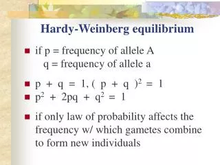
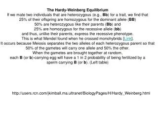
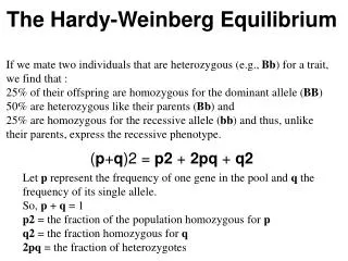
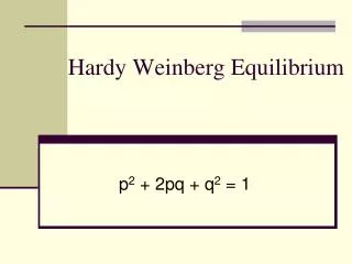
11.4 Hardy-Weinberg Equilibrium "The Hardy-Weinberg equation is based on Mendelian genetics. It is derived from a simple Punnett square in which p is the frequency of the dominant allele and q is the frequency of the recessive allele." Equation - used to predict genotype frequencies in a population • Predicted genotype frequencies are compared withActual frequencies • used for traits in simple dominant-recessive systems p2 + 2pq + q2 = 1
11.4 Hardy-Weinberg Equilibrium • q2 = # homozygous recessive/entire population • p2 = # homozygous dominant/entire population • Take the square roots to find p & q • If the predicted genotypes match the actual genotype frequencies than population is in equilibrium • If it is not in equilibrium • it is changing - evolving
Chi-Square Test • Determines whether the experimental data fits the results expected • For example • 290 purple flowers • 110 white flowers • Close to a 3 : 1 ratio • How do you know for sure?
Goodness of Fit • The chi-square test is a “goodness of fit” test • Answers the question of how well do experimental data fit expectations • Ex: self-pollination of a heterozygote • The null hypothesis is that the offspring will appear in a ratio of 3 dominant to 1 recessive.
Formula • First determine the number of each phenotype that have been observed and how many would be expected • “Χ” - Greek letter chi • “∑” - sigma • Sum the following terms for all phenotypes • “obs” is the number of individuals of the given phenotype observed • “exp” is the number of that phenotype expected from the null hypothesis • Must use the number of individualsand NOT proportions, ratios, or frequencies
Example • F2 offspring • 290 purple and 110 white flowers • Total of 400 offspring • We expect a 3 : 1 ratio. • To calculate the expected numbers • Multiply the total offspring by the expected proportions • Expected Purple = 400 * 3/4 = 300 purple • Expected White = 400 * 1/4 = 100 white
Purple obs = 290 and exp = 300 • White obs = 110 and exp = 100 • Plug into the formula: 2 = (290 - 300)2 / 300 + (110 - 100)2 / 100 = (-10)2 / 300 + (10)2 / 100 = 100 / 300 + 100 / 100 = 0.333 + 1.000 = 1.333 • = chi-square value
Reasonable • What is a “reasonable” result is subjective and arbitrary • For most work a result is said to not differ significantly from expectations if it could happen at least 1 time in 20 • That is, if the difference between the observed results and the expected results is small enough that it would be seen at least 1 time in 20 over thousands of experiments • “1 time in 20” can be written as a probability value p = 1/20 = 0.05
Degrees of Freedom • The number of independent random variables involved • Simply the number of classes of offspring minus 1 • Example: • 2 classes of offspring: purple and white • Degrees of freedom (d.f.) = 2 -1 = 1.
Critical Chi-Square • Critical values for chi-square are found on tables, sorted by degrees of freedom and probability levels • If your calculated chi-square value is greater than the critical value from the table, you “reject the null hypothesis” • If your chi-square value is less than the critical value, you “fail to reject” the null hypothesis • Accept that your genetic theory about the expected ratio is correct
Using the Table • Example of 290 purple to 110 white • Chi-square value of 1.333, with 1 degree of freedom • 1 d.f. is the first row, and p = 0.05 is the sixth column • Critical chi-square value = 3.841 • Calculated chi-square = 1.333 • less than the critical value, 3.841 • “fail to reject” the null hypothesis • An observed ratio of 290 purple to 110 white is a good fit to a 3 to 1 ratio
Finding the Expected Numbers • Add up the observed offspring to get the total number of offspring • Example: 315 + 101 + 108 + 32 = 556 • Multiply total offspring by the expected proportion --expected round yellow = 9/16 * 556 = 312.75 --expected round green = 3/16 * 556 = 104.25 --expected wrinkled yellow = 3/16 * 556 = 104.25 --expected wrinkled green = 1/16 * 556 = 34.75
Calculating the Chi-Square Value X2= (315 - 312.75)2 / 312.75 + (101 - 104.25)2 / 104.25 + (108 - 104.25)2 / 104.25 + (32 - 34.75)2 / 34.75 = 0.016 + 0.101 + 0.135 + 0.218 = 0.470.
D.F. and Critical Value • Degrees of freedom • 4 - 1 = 3 d.f. • 3 d.f. and p = 0.05 • critical chi-square value = 7.815 • Observed chi-square (0.470) is less than the critical value • Fail to reject the null hypothesis • Accept Mendel’s conclusion that the observed results for a 9/16 : 3/16 : 3/16 : 1/16 ratio