Download
1 / 35
350 likes | 467 Views
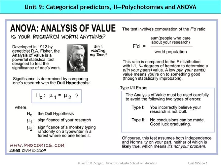
Unit 9: Categorical predictors, II—Polychotomies and ANOVA. The S-030 roadmap: Where’s this unit in the big picture?. Unit 1: Introduction to simple linear regression. Unit 2: Correlation and causality. Unit 3: Inference for the regression model. Building a solid foundation.

E N D
The S-030 roadmap: Where’s this unit in the big picture? Unit 1: Introduction to simple linear regression Unit 2: Correlation and causality Unit 3: Inference for the regression model Building a solid foundation Unit 5: Transformations to achieve linearity Unit 4: Regression assumptions: Evaluating their tenability Mastering the subtleties Adding additional predictors Unit 6: The basics of multiple regression Unit 7: Statistical control in depth: Correlation and collinearity Generalizing to other types of predictors and effects Unit 9: Categorical predictors II: Polychotomies Unit 8: Categorical predictors I: Dichotomies Unit 10: Interaction and quadratic effects Pulling it all together Unit 11: Regression modeling in practice
In this unit, we’re going to learn about… • Distinguishing between nominal and ordinal predictors • How a series of 0/1 dummy variables can represent a nominal predictor • Why does regressing Y on all but one dummy variable yield the desired model? • Consequences of changing the reference category for parameter estimates and hypothesis tests • The problem of multiple comparisons: How many contrasts have we examined? • The Bonferroni multiple comparison procedure: Splitting the p-value • An alternative way of getting the identical results: The analysis of variance (ANOVA) • What else might we do if we have an ordinal predictor? • Presenting adjusted means when the question predictor is polychotomous • Untangling the nomenclature: Regression, analysis of variance and analysis of covariance
Distinguishing between nominal and ordinal predictors Nominal predictors Variables whose values offer no meaningful quantitative information but simply distinguish between categories Ordinal predictors Variables whose values do reflect an underlying ordering of categories, but not necessarily the “distance” between categories You can directly include an ordinal predictor in a regression model, but be sure that’s what you want. It’s often not! Never directly include a nominal predictor in a regression model. Never!
Regional differences in the price of fine French wine Source: Thrane, C (2004). In defence of the price hedonic model in wine research, Journal of Wine Research, 15(2), 123-134 n = 113 Ordinal Nominal ID Region Area Price Lprice Year Vintage 3 2 Bordeaux 13.2286 2.58238 3 2001 109 4 Languedoc 13.2571 2.58454 2 2000 110 4 Languedoc 13.4286 2.59738 3 2001 131 3 Rhone 13.4429 2.59845 3 2001 133 3 Rhone 13.5000 2.60269 1 1999 111 4 Languedoc 13.5571 2.60691 3 2001 61 1 Burgundy 14.1286 2.64820 3 2001 . . . 57 2 Bordeaux 47.0714 3.85167 0 1998(-) 58 2 Bordeaux 50.1429 3.91488 0 1998(-) 178 1 Burgundy 52.6429 3.96353 2 2000 160 3 Rhone 52.9000 3.96840 2 2000 183 1 Burgundy 62.9571 4.14245 3 2001 60 2 Bordeaux 66.4000 4.19570 2 2000 RQ 1: Do wine prices vary (significantly) by region and vintage? RQ 2: If so, which regions and vintages are (significantly) different from which other regions and vintages?
How do wine prices vary by REGION? Languedoc Burgundy Bordeaux Rhone mean 3.39 3.25 3.06 2.65 Much variability between regions: Burgundy is most expensive, on average You can buy a “cheap” (for Norway…) bottle from anywhere: e.g., each region’s range includes Lprice ≈ 2.75 (~$15) That said, there’s great variability withinregions Is there heteroscedasticity? SD’s vary: highest (.48) is 2.5 times higher than the lowest (.19) (sd) (0.48) (0.40) (0.36) (0.19)
How do wine prices vary by VINTAGE? 2001 <= ‘98 1999 2000 mean 3.46 3.20 3.13 2.85 • Two Qs we want to ask about group differences: • How much credence should we give to observed differences between group means? • In what context can we place these observed differences to evaluate their magnitude? Much variability between vintages: On average, older wines are more expensive than younger ones You can buy a “cheap” (for Norway…) bottle from any vintage: each vintage’s range includes Lprice ≈ 2.75 (~$15) That said, there’s great variability withinvintages Less heteroscedasticity? SD’s still vary but appear more stable (with sd’s ≈ .40) (sd) (0.34) (0.41) (0.43) (0.37)
Why within-group variance is key to evaluating between-group differences † † † † † † † † † † † † How much attention would you give to these observed group-to-group differences in means… Let’s imagine 3 different data sets for a 4-level categorical predictor where the set of 4 means is identical in each Important message: Within-group variation provides a key context for evaluating the magnitude of between-group variation …if there were equally little variability within groups? …if there were equally moderate variability within groups? …if there were equally great variability within groups?
Towards postulating a statistical model for group differences 2001 <= ‘98 1999 2000 Languedoc Burgundy Bordeaux Rhone mean 3.46 3.20 3.13 2.85 mean 3.39 3.25 3.06 2.65 (sd) (0.48) (0.40) (0.36) (0.19) (sd) (0.34) (0.41) (0.43) (0.37) Regional variation Vintage variation We seek a statistical model that includes the effects of categorical predictors in a way that is similar to regression (in that its parameters represent population means) but thatdoesn’t force us to hypothesize the existence of a linear relationship What happens if we incorrectly include REGION as a continuous predictor?
How do we include a polychotomy in a regression model?Creating a series of 0/1 dummy variables Collectively, the 4 dummies identify every wine’s specific region But 3 dummies would also be sufficient to identify every wine’s specific region! Because the Y-intercept is value of Y when all predictors = 0 it represents the mean outcome for the reference category Step One: Create a series of 0/1 dummy variables, one for every value of the categorical predictor ID LPrice Region Area 61 2.64820 1 Burgundy 66 3.00285 1 Burgundy 67 3.00498 1 Burgundy 72 3.67449 1 Burgundy 178 3.96353 1 Burgundy 7 2.65826 2 Bordeaux 48 3.70658 2 Bordeaux 53 3.75754 2 Bordeaux 55 3.79324 2 Bordeaux 56 3.81991 2 Bordeaux 146 2.99502 3 Rhone 145 2.99502 3 Rhone 151 3.20100 3 Rhone 152 3.22457 3 Rhone 154 3.40120 3 Rhone 119 2.71753 4 Languedoc 120 2.75366 4 Languedoc 122 2.84075 4 Languedoc 127 2.96674 4 Languedoc 180 2.96821 4 Languedoc Burgundy 1 1 1 1 1 0 0 0 0 0 0 0 0 0 0 0 0 0 0 0 Rhone 0 0 0 0 0 0 0 0 0 0 1 1 1 1 1 0 0 0 0 0 Languedoc 0 0 0 0 0 0 0 0 0 0 0 0 0 0 0 1 1 1 1 1 Bordeaux 0 0 0 0 0 1 1 1 1 1 0 0 0 0 0 0 0 0 0 0 These 3 dummies are mutually exclusive and exhaustive Step Two: Include all but one of the dummy variables in the multiple regression model (for K groups, you need only K-1 dummies)
Why does regressing Y on all but one dummy yield our postulated model?
Results of regressing LPrice on 3 regional dummies (Burgundy, Bordeaux and Rhone—Languedoc is the reference category) Wine prices vary significantly by region. We reject H0: 1 = 2= 3 = 0 at the p<.0001 level. (Note that this is now a very interesting test.) To side by side boxplots RMSE estimates the average within-group standard deviation Region “explains” just over 1/3 of the variation in price (R2=36.2%) The intercept provides the estimated mean for the reference category: The estimated mean log(price) for Languedoc wines is 2.65 The REG Procedure Dependent Variable: Lprice Analysis of Variance Sum of Mean Source DF Squares Square F Value Pr > F Model 3 7.88009 2.62670 20.62 <.0001 Error 109 13.88838 0.12742 Corrected Total 112 21.76847 Root MSE 0.35695 R-Square 0.3620 Dependent Mean 3.06102 Adj R-Sq 0.3444 Coeff Var 11.66128 Parameter Estimates Parameter Standard Variable DF Estimate Error t Value Pr > |t| Intercept 1 2.64606 0.06517 40.60 <.0001 Burgundy 1 0.74061 0.13566 5.46 <.0001 Bordeaux 1 0.60072 0.08213 7.31 <.0001 Rhone 1 0.41690 0.09893 4.21 <.0001 Each regression coefficient estimates the differential between the mean of that group and the mean of the reference group (NOT the overall mean): The estimated mean log(price) of each region’s wine is significantly higher than that of the Languedoc (p<.0001)… BUT we don’t yet know if there are significant price differences between Burgundy and Rhone, Rhone and Bordeaux, etc.
Relating the fitted model to the sample data Interpretation of estimates for categorical predictors depends, then, on choice of the reference category... So choose your reference category wisely Parameter estimate for each dummy variable = in means between this category and the reference category (e.g., we estimate that the mean difference in Lprice between Burgundy and the Languedoc is 0.74, which is the difference between 3.39 and 2.65) estimated difference 3.39 3.25 3.06 2.65 estimated mean for the reference category (e.g,. the estimated mean for the Languedoc is 2.65)
What happens if we change the model’s “reference category”? Reference Category: Languedoc Parameter Standard Variable DF Estimate Error t Value Pr > |t| Intercept 1 2.64606 0.06517 40.60 <.0001 Burgundy 1 0.74061 0.13566 5.46 <.0001 Bordeaux 1 0.60072 0.08213 7.31 <.0001 Rhone 1 0.41690 0.09893 4.21 <.0001 Reference Category: Rhone Parameter Standard Variable DF Estimate Error t Value Pr > |t| Intercept 1 3.06296 0.07443 41.15 <.0001 Burgundy 1 0.32372 0.14035 2.31 0.0230 Bordeaux 1 0.18382 0.08966 2.05 0.0427 Languedoc 1 -0.41690 0.09893 -4.21 <.0001 Reference Category: Bordeaux Parameter Standard Variable DF Estimate Error t Value Pr > |t| Intercept 1 3.24678 0.04998 64.96 <.0001 Burgundy 1 0.13990 0.12906 1.08 0.2808 Rhone 1 -0.18382 0.08966 -2.05 0.0427 Languedoc 1 -0.60072 0.08213 -7.31 <.0001 Reference Category: Burgundy Parameter Standard Variable DF Estimate Error t Value Pr > |t| Intercept 1 3.38667 0.11898 28.46 <.0001 Bordeaux 1 -0.13990 0.12906 -1.08 0.2808 Rhone 1 -0.32372 0.14035 -2.31 0.0230 Languedoc 1 -0.74061 0.13566 -5.46 <.0001
Understanding the consequences of changing the reference category on estimated regression coefficients and hypothesis tests RQ 1: Do wine prices vary (significantly) by region? RQ 2: If so, which regions are (significantly) different from which other regions? The intercept is always the estimated mean of Y in the reference category Parameter estimates (& associated tests) for each dummy variable will change because they always refer to the estimated difference between the mean for that group and the mean for that model’s ref category. Even though there’s significant variation between regions, not all regions are significantly different from each other The estimate and associated test for all specific contrasts remain the same (although the sign will change to reflect the reversal of the contrast’s direction) YES: F(3,109)=20.62, p<0.0001 Are we sure that we know?
The problem of multiple comparisons: How many contrasts have we examined & taken together, should we ‘believe’ all these tests? We focus on minimizing Type I error when we set p=0.05 for our tests, but as we conduct multiple tests, the Type I error for the “family of tests” grows Two types of errors we can make every time we conduct a hypothesis test: Type I error: Rejecting H0 when it’s true—saying there’s a difference in means when there isn’t Type II error: Failing to reject H0 when it’s false—saying we can’t find a difference in means when there really is one Idea: Instead of using p=0.05 for each individual test, why not use p=0.05 for the entire family of tests when we examine multiple contrasts to test a single hypothesis
Multiple comparison procedures: What they are and how they’re used SurfStat t-distribution calculator New p-value and associated t-statistic to use the Bonferroni method to keep the “family error rate” at 0.05 (two-tailed tests) # tests New p New t-statistic df=50 df=100 df= 1 0.0500 2.01 1.98 1.96 2 0.0250 2.31 2.28 2.24 3 0.0167 2.48 2.43 2.39 4 0.0125 2.59 2.54 2.50 5 0.0100 2.68 2.63 2.58 6 0.0083 2.75 2.69 2.64 10 0.0050 2.94 2.87 2.81 20 0.0025 3.18 3.10 3.02 50 0.0010 3.50 3.39 3.29 100 0.0005 3.72 3.60 3.48 • Some multiple comparison procedures: • Duncan’s Multiple Range Test • Tukey’s Honest Significant Difference • Scheffe’s Multiple Comparison Test • Newman Keuls Multiple Comparison Test • Benjamini & Hochberg • …. many more, including … • Bonferroni’s method • Issues involved in selecting an approach: • A priori or post-hoc comparison? • Simple or complex comparison? • Is there a clearly identified control group? • Equal or unequal n’s within groups? • The Bonferroni approach: • Take a chosen Type I error rate (usually 0.05) and “split it” across the entire family of tests you’re conducting • For 2 tests, conduct each at the 0.025 level • For 5 tests, conduct each at the 0.01 level • Use this new p-value to identify the new t-statistic for testing each individual hypothesis in the family, for a given number of degrees of freedom As # of tests increases, critical t-values increase. As DF increase, critical t-values decrease.
Applying Bonferroni multiple comparisons to regional variation in wine prices RQ 2: If so, which regions are (significantly) different from which other regions? Only the Languedoc is significantly different from all 3 others The mean Languedoc price is still significantly different from that of Burgundy, Bordeaux and the Rhone What changes: The mean Rhone price is now indistinguishable from that of Burgundy and Bordeaux Critical t = 2.69, p<.0.0083 (from previous slide’s table) The mean Bordeaux price is still indistinguishable from that of Burgundy (note: a test that didn’t reject on its own will never reject after using a multiple comparison procedure)
An alternative way of getting the identical multiple regression results: The analysis of variance (ANOVA) obtained in SAS using PROC GLM PROC GLM stands for the General Linear Model, which is SAS’ procedure for conducting an analysis of variance (ANOVA), the results of which we already obtained using PROC REG The GLM Procedure Least Squares Means Adjustment for Multiple Comparisons: Bonferroni Lprice LSMEAN Region LSMEAN Number 1 3.38667410 1 2 3.24677775 2 3 3.06295573 3 4 2.64606047 4 Least Squares Means for Effect Region t for H0: LSMean(i)=LSMean(j) / Pr > |t| Dependent Variable: Lprice i/j 1 2 3 4 1 1.083988 2.306561 5.459197 1.0000 0.1378 <.0001 2 -1.08399 2.050303 7.314098 1.0000 0.2564 <.0001 3 -2.30656 -2.0503 4.214063 0.1378 0.2564 0.0003 4 -5.4592 -7.3141 -4.21406 <.0001 <.0001 0.0003 The GLM Procedure Dependent Variable: Lprice Sum of Source DF Squares Mean Square F Value Pr > F Model 3 7.88008697 2.62669566 20.62 <.0001 Error 109 13.88837973 0.12741633 Corrected Total 112 21.76846670 R-Square Coeff Var Root MSE Lprice Mean 0.361995 11.66128 0.356954 3.061022 Standard Parameter Estimate Error t Value Pr > |t| Intercept 2.646060467 B 0.06517063 40.60 <.0001 Region 1=Burgundy 0.740613638 B 0.13566348 5.46 <.0001 Region 2=Bordeaux 0.600717281 B 0.08213142 7.31 <.0001 Region 3=Rhone 0.416895264 B 0.09892953 4.21 <.0001 Region 4=Languedoc 0.000000000 B . . . NOTE: The X'X matrix has been found to be singular, and a generalized inverse was used to solve the normal equations. Terms whose estimates are followed by the letter'B' are not uniquely estimable.
Multiple comparisons in practice, I: Astrological signs and health Hypothesis generating sample (n=5,333,472) Hypothesis validation sample (n=5,333,473) Austin et al (2006) Journal of Clinical Epidemiology, 59, 964-969 Studied all 10,674,945 residents of Ontario, between 18 and 100 in 2000 • Studied the 223 diagnoses (e.g., neck fracture, heart failure etc) that accounted for over 90% of all hospitalizations in the region • Question predictor: Astrological sign (which has 12 categories) • Of these 223 diagnoses, there were 72 (32.3%) for which residents from one astrological sign had a significantly higher probability of hospitalization (p’s ranging from 0.0003 to 0.0488); these focused on 24 diagnoses • Lowest p value (.0006) for Taurus being 27% more likely to have diverticula of intestine. FYI, Capricorns were 28% more likely to have abortions • Studied the 24 diagnoses in this second sample; only 2 associations remained statistically significant • Leos were 15% more likely to be hospitalized for gastrointestinal hemorrhage (p=0.0483); Saggitarians were 38% more likely to have fractures of the humerus (p=0.0125) With 12 astrological signs: (12*11)/2 = 66 contrasts per diagnosis, which adds up to 14,718 comparisons across the 223 diagnoses p = 0.000003485 t= 4.64 If they had adjusted for multiple comparisons, none of these tests would have rejected either If they had adjusted for multiple comparisons, none of these 72 tests would have rejected
Multiple comparisons in practice, II: PISA international comparisons With 29 countries: (29*28)/2 = 406 contrasts p = 0.000124 t= 3.84 Source: OECD (2005) Education at a Glance What's wrong with Bonferroni adjustments British Medical Journal 1998;316:1236-1238In controlling your overall Type I error, you’re inevitably increasing your Type II error—that is, decreasing your statistical power
How do we handle an ordinal categorical predictor like Vintage? Collectively, the 4 dummies identify every wine’s specific vintage But 3 dummies would still be sufficient to identify every wine’s specific vintage! Step One: Create a series of 0/1 dummy variables, one for every value of the categorical predictor ID Lprice Year VINTAGE 4 2.65525 0 <= '98 19 3.06606 0 <= '98 22 3.11605 0 <= '98 50 3.70658 0 <= '98 53 3.75754 0 <= '98 119 2.71753 1 '99 124 2.85400 1 '99 157 3.55126 1 '99 46 3.63646 1 '99 56 3.81991 1 '99 13 2.88080 2 '00 141 2.88240 2 '00 155 3.48781 2 '00 182 3.49391 2 '00 158 3.69102 2 '00 122 2.84075 3 '01 20 3.08257 3 '01 150 3.11668 3 '01 42 3.55494 3 '01 45 3.59103 3 '01 Yr98 1 1 1 1 1 0 0 0 0 0 0 0 0 0 0 0 0 0 0 0 Yr00 0 0 0 0 0 0 0 0 0 0 1 1 1 1 1 0 0 0 0 0 Yr01 0 0 0 0 0 0 0 0 0 0 0 0 0 0 0 1 1 1 1 1 Yr99 0 0 0 0 0 1 1 1 1 1 0 0 0 0 0 0 0 0 0 0 Step Two: Include all but one of the dummy variables in the multiple regression model
Results of regressing LPrice on 3 vintage dummies (Yr98, Yr99 and Yr01—Yr01 is the reference category) Wine prices vary significantly by vintage. We can reject H0: 1 = 2= 3 = 0 at the p<.0001 level To side by side boxplots RMSE estimates the average within-group standard deviation Vintage “explains” ¼ of the variation in price (R2=24.0%) The intercept provides the estimated mean for the reference category: The estimated mean log(price) for wines from 2001 is 2.85 The regression coefficient for each dummy variable estimates the mean differential between that group and the reference category: The estimated mean log(price) of wines from all other vintages is significantly higher than that of wines from 2001 The REG Procedure Dependent Variable: Lprice Analysis of Variance Sum of Mean Source DF Squares Square F Value Pr > F Model 3 5.21329 1.73776 11.44 <.0001 Error 109 16.55518 0.15188 Corrected Total 112 21.76847 Root MSE 0.38972 R-Square 0.2395 Dependent Mean 3.06102 Adj R-Sq 0.2186 Coeff Var 12.73172 Parameter Estimates Parameter Standard Variable DF Estimate Error t Value Pr > |t| Intercept 1 2.84676 0.05567 51.13 <.0001 yr98 1 0.61424 0.11222 5.47 <.0001 yr99 1 0.35472 0.12158 2.92 0.0043 yr00 1 0.27921 0.08625 3.24 0.0016
What about multiple comparisons for the vintage means? 3.75 3.50 3.25 3.00 2.75 2.50 1997 1998 1999 2000 2001 2002 The GLM Procedure Least Squares Means Adjustment for Multiple Comparisons: Bonferroni Lprice LSMEAN Vintage LSMEAN Number 1998(-) 3.46100054 1 1999 3.20148133 2 2000 3.12596879 3 2001 2.84676233 4 Least Squares Means for Effect Vintage t for H0: LSMean(i)=LSMean(j) / Pr > |t| Dependent Variable: Lprice i/j 1 2 3 4 1 1.783399 2.848664 5.473744 0.4638 0.0315 <.0001 2 -1.7834 0.596555 2.917458 0.4638 1.0000 0.0257 3 -2.84866 -0.59655 3.23716 0.0315 1.0000 0.0096 4 -5.47374 -2.91746 -3.23716 <.0001 0.0257 0.0096 Do the estimated means for the ordinal predictor seem to follow a pattern? The mean price for 2001 is significantly different from all earlier vintages Go back to dataset 2000 is distinguishable from 1998 Aside from the’00/’01 contrast, adjacent vintages are indistinguishable
What happens when we use continuous YEAR instead of Vintage dummies? Region effects controlling for continuous Year Root MSE 0.33243 R-Square 0.4517 Dependent Mean 3.06102 Adj R-Sq 0.4314 Coeff Var 10.86008 Parameter Estimates Parameter Standard Variable DF Estimate Error t Value Pr > |t| Intercept 1 3.00062 0.10390 28.88 <.0001 Year 1 -0.13814 0.03286 -4.20 <.0001 Burgundy 1 0.67768 0.12723 5.33 <.0001 Bordeaux 1 0.46014 0.08348 5.51 <.0001 Rhone 1 0.39267 0.09231 4.25 <.0001 Treating YEAR as a categorical predictor Root MSE 0.38972 R-Square 0.2395 Dependent Mean 3.06102 Adj R-Sq 0.2186 Coeff Var 12.73172 Parameter Estimates Parameter Standard Variable DF Estimate Error t Value Pr > |t| Intercept 1 3.46100 0.09743 35.52 <.0001 yr99 1 -0.25952 0.14552 -1.78 0.0773 yr00 1 -0.33503 0.11761 -2.85 0.0052 yr01 1 -0.61424 0.11222 -5.47 <.0001 Treating YEAR as a continuous predictor Root MSE 0.38850 R-Square 0.2304 Dependent Mean 3.06102 Adj R-Sq 0.2235 Coeff Var 12.69172 Parameter Estimates Parameter Standard Variable DF Estimate Error t Value Pr > |t| Intercept 1 3.46733 0.07940 43.67 <.0001 Year 1 -0.19962 0.03463 -5.76 <.0001 Bonferroni multiple comparisons for REGION controlling for continuous Year Lprice LSMEAN Region LSMEAN Number 1 3.39713319 1 2 3.17958869 2 3 3.11212112 3 4 2.71945067 4 Least Squares Means for Effect Region t for H0: LSMean(i)=LSMean(j) / Pr > |t| Dependent Variable: Lprice i/j 1 2 3 4 1 1.789005 2.1752 5.326594 0.4585 0.1908 <.0001 2 -1.789 0.766998 5.512103 0.4585 1.0000 <.0001 3 -2.1752 -0.767 4.253707 0.1908 1.0000 0.0003 4 -5.32659 -5.5121 -4.25371 <.0001 <.0001 0.0003 To uncontrolled Bonferroni comparisons for Region
How might we present the results of this analysis? Loge(Price) Burgundy Bordeaux Rhone Languedoc Vintage The only statistically significant difference in regional means, after linearly controlling for vintage, is between the Languedoc and all others Regression results predicting the loge(price) of French wine by vintage and region (Languedoc is the omitted category) Model A Model B Model C Intercept 2.65*** (0.07) 3.46*** (0.08) 3.00*** (0.10) Vintage (linear year) -0.20*** (0.03) -0.14*** (0.03) Burgundy 0.74*** (0.14) 0.68*** (0.13) Bordeaux 0.60*** (0.08) 0.46*** (0.08) Rhone 0.42*** (0.10) 0.39*** (0.09) R2 36.2 23.0 45.2 F df P 20.62 (3,109) <0.0001 33.23 (1,111) <0.0001 22.25 (4,108) <0.0001 Cell entries are estimated regression coefficients and standard errors. ***p<0.0001
Supplemental presentation of adjusted means Burgundy 3.40 Bordeaux 3.18 Rhone 3.11 Languedoc 2.72 Controlling for vintage Loge(Price) Year 0 1 2 3 (n) (16) (13) (35) (49)
A word about nomenclature: Regression, GLM, ANOVA and ANCOVA General Linear Model Initially developed to measure treatment effects in designed experiments (ideally using a balanced—equal n—design) Initially developed for observational studies & sample surveys and can be applied to designed experiments Initially developed to measure treatment effects in a quasi-experiment with a covariate Early adopters: Educational and medical researchers Early adopters: Psychologists and agricultural researchers Early adopters: Sociologists and economists Regression Model Analysis of Variance Statistical model relating categorical predictors to a continuous outcome Analysis of Covariance Statistical model relating categorical predictors to a continuous outcome, controlling for one or more covariates Regression Statistical model relating continuous and categorical predictors to a continuous outcome
A ‘standard’ psychology dept presentation of these methods David Howell, Statistical Methods for Psychology
A ‘standard’ economics dept presentation of these methods Peter Kennedy, A Guide to Econometrics
What’s the big takeaway from this unit? • Regression models can easily include polychotomies • Once you know how to include dichotomous predictors, its easy to extend this strategy to polychotomous predictors • Can be used for either nominal or ordinal predictors • Make a wise decision about the omitted (reference) category—results are most easily interpreted if it provides an interesting/important comparison • Understand the issues associated with conducting multiple hypothesis tests • The more predictors you have, the more models you fit, and the more hypothesis tests you conduct • Don’t fall into the trap of strictly interpreting p-values and consider correcting for the multiplicity of tests • Analysis of variance is just a special case of multiple regression • There’s nothing mysterious about ANOVA; it’s just regression on dummy variables • By learning regression, you’re learning the more general approach, of which classical ANOVA is just a special case
Appendix: Annotated PC-SAS Code for Using Polychotomies *-------------------------------------------------------------------* Input Wine data and name variables in dataset Create transformation of outcome variable PRICE Create dummy coding system for REGION/AREA and YEAR/VINTAGE *------------------------------------------------------------------*; data one; infile "m:\datasets\wine.txt"; input ID 1-3 Price 5-16 Region 19 Area $ 21-31 Year 34 Vintage $ 38-44 Rating 48-51; Lprice = log(price); if Region = 1 then Burgundy=1; else Burgundy=0; if Region = 2 then Bordeaux=1; else Bordeaux=0; if Region = 3 then Rhone=1; else Rhone=0; if Region = 4 then Languedoc=1; else Languedoc=0; if year=0 then yr98=1; else yr98=0; if year=1 then yr99=1; else yr99=0; if year=2 then yr00=1; else yr00=0; if year=3 then yr01=1; else yr01=0; The data stepincludes code that takes the two polychotomies (Region and Year) and creates a series of 0/1 indicator variables (dummy variables) for each, The if-then-else statement specifies which categories of the polychotomies identifies the relevant categories for the new indicator variables. proc glmis SAS’ general linear model and procedure and is an easy way to fit an analysis of variance (ANOVA) model. For our purposes here, its greatest value is the simplicity with which it does multiple comparisons test. The lsmeans region/adjust=bon statement tells SAS to output Bonferroni multiple comparisons (here, by region) with adjusted t-statistics and p-values. *-------------------------------------------------------------------* Fitting a general linear model LPRICE by REGION (ANOVA approach using PROC GLM) with Bonferroni multiple comparisons *------------------------------------------------------------------*; procglm data=one; title2 "Demonstrating the equivalence of ANOVA and regression"; class region; model lprice = region/solution; lsmeans region/adjust=bon tdiff pdiff;
Glossary terms included in Unit 9 • Categorical predictor • Dummy variables • Multiple comparisons • Polychotomous predictor • Type I and Type II error
Appendix: Incorrectly including REGION as a continuous predictor Regression results with REGION as a continuous predictor--INCORRECT, OF COURSE The REG Procedure Model: MODEL1 Dependent Variable: Lprice Number of Observations Read 113 Number of Observations Used 113 Analysis of Variance Sum of Mean Source DF Squares Square F Value Pr > F Model 1 7.45565 7.45565 57.82 <.0001 Error 111 14.31281 0.12894 Corrected Total 112 21.76847 Root MSE 0.35909 R-Square 0.3425 Dependent Mean 3.06102 Adj R-Sq 0.3366 Coeff Var 11.73099 Parameter Estimates Parameter Standard Variable DF Estimate Error t Value Pr > |t| Intercept 1 3.77344 0.09959 37.89 <.0001 Region 1 -0.26834 0.03529 -7.60 <.0001
Appendix: What happens if you include all 4 REGIONAL dummies? Regression results with including 4 REGIONAL dummies The REG Procedure Model: MODEL1 Dependent Variable: Lprice Analysis of Variance Sum of Mean Source DF Squares Square F Value Pr > F Model 3 7.88009 2.62670 20.62 <.0001 Error 109 13.88838 0.12742 Corrected Total 112 21.76847 Root MSE 0.35695 R-Square 0.3620 Dependent Mean 3.06102 Adj R-Sq 0.3444 Coeff Var 11.66128 NOTE: Model is not full rank. Least-squares solutions for the parameters are not unique. Some statistics will be misleading. A reported DF of 0 or B means that the estimate is biased. NOTE: The following parameters have been set to 0, since the variables are a linear combination of other variables as shown. Rhone = Intercept - Languedoc - Burgundy - Bordeaux Parameter Estimates Parameter Standard Variable DF Estimate Error t Value Pr > |t| Intercept B 3.06296 0.07443 41.15 <.0001 Languedoc B -0.41690 0.09893 -4.21 <.0001 Burgundy B 0.32372 0.14035 2.31 0.0230 Bordeaux B 0.18382 0.08966 2.05 0.0427 Rhone 0 0 . . .