Download
1 / 30
300 likes | 394 Views
Downscaling for the World of Water. E.P. Maurer Santa Clara University, Civil Engineering Dept. NCPP Workshop Quantitative Evaluation of Downscaling 12-16 August, 2013 Boulder, CO. Extending hydrology to include climate change seems easy…. Estimating Climate Impacts to Water.

E N D
Downscaling for the World of Water E.P. Maurer Santa Clara University, Civil Engineering Dept. NCPP Workshop Quantitative Evaluation of Downscaling 12-16 August, 2013 Boulder, CO
Estimating Climate Impacts to Water 2. Global Climate Model 4. Land surface (Hydrology) Model 1. GHG Emissions Scenario 5. Operations/impacts Models • “Downscaling” Adapted from Cayan and Knowles, SCRIPPS/USGS, 2003
Downscaling: bringing global signals to regional scale GCM scale and processes at too coarse a scale Figure: Wilks, 1995 • Resolved by: • Bias Correction • Spatial Downscaling
IPCC CMIP3 GCM Simulations • 20th century through 2100 and beyond • >20 GCMs • Multiple Future Emissions Scenarios http://www-pcmdi.llnl.gov/
2/3 chance that loss will be at least 40% by mid century, 70% by end of century Point at: 120ºW, 38ºN Impact Probabilities for Planning Snow water equivalent on April 1, mm • Combine many future scenarios, models, since we don’t know which path we’ll follow (22 futures here) • Choose appropriate level of risk
Incorporating probabilistic projections into water planning • Overdesign for present • Can represent declining return periods for extreme events Das et al, 2012 Mailhot and Sophie Duchesne, JWRPM, 2010
Monthly downscaled data • PCMDI CMIP3 archive of global projections • 16 GCMs, 3 Emissions • 112 GCM runs • Allows quick analysis of multi-model ensembles • gdo4.ucllnl.org/downscaled_cmip3_projections
Use of U.S. Data Archive • Thousands of users downloaded >20 TB of data • Uses for Research (R), Management & Planning (MP), Education (E)
Downscaling for Extreme Events • Some impacts due to changes at short time scales • Heat waves • Flood events • Daily GCM output limited for CMIP3, more plentiful for CMIP5 • Downscaling adapted for modeling extremes
Archive expansion • Daily downscaled data (BCCA) • Hydrology model output • CMIP5
Online Analysis and Download withhttp://ClimateWizard.org • Global and US data sets • Country and US state boundaries defined • Spatial and time series analysis • Ensemble quick view • Upload of custom shapefiles Girvetz et al., PLoS, 2009
Information Overload (practitioner’s dilemma) • Little guidance in selection of: • Emissions • GCMs • Downscaling methods • Hundreds of downscaled GCM runs • Many impacts studies cannot use all of them • How much information is really useful?
Selecting 4 Specific GCM Runs • Bivariate probability plot shows correlation between T, P • Identify Change Range: 10 to 90 %-tile T, P • Select bounds based on: • risk attitude • interest in breadth of changes • number of simulations desired Brekke et al., 2009
Selecting GCMs for Impact Studies • Ensemble mean provides better skill • Little advantage to weighting GCMs according to skill • Most important to have “ensembles of runs with enough realizations to reduce the effects of natural internal climate variability” [Pierce et al., 2009] • Maybe 10-14 GCMs is enough? Gleckler, Taylor, and Doutriaux, Journal of Geophysical Research (2008) as adapted by B. Santer Brekke et al., 2008
Discard CMIP3 in favor of CMIP5? • Ensemble average changes comparable • RCP8.5 and SRES A2 comparable
Is BCSD method valid? • At each grid cell for “training” period, develop monthly CDFs of P, T for • GCM • Observations (aggregated to GCM scale) • Obs are from Maurer et al. [2002] • Use quantile mapping to ensure monthly statistics (at GCM scale) match obs • Apply same quantile mapping to “projected” period Wood et al., BAMS 2006
Are biases time-invariant? Biases vary in time, space, at quantiles R index: compares size of bias variability to average GCM bias
Time-invariant enough… • On average, time-invariant enough where bias correction works • But for small ensembles maybe not (locations where biases vary with time differ for GCMs)
Bias correction changes trends! Raw GCM Bias Corrected • Changes in mean annual precipitation: 1970-1999 to 2040-2069 • Similar effect in CMIP3 and CMIP5 • Some more intense wettening in Rockies for CMIP5
What happens? • Contrived Example (Precipitation): • Gamma distributions • asymmetry • Obs: mean=30 • GCM Historic has −30% bias in SD • GCM future has +40% change in mean
What is effect of trend/shift? • Quantile mapping changes shift in mean • +40% becomes +56% • -40% becomes -39% • 5% decrease changes to ~2% increase
But is changing the trend bad? • estimated change in precip from 1916-1945 and 1976-2005. • Where index is >1 BC worsens • Ensemble avg shows trend modification not consistently bad. Ensemble Avg
Challenges in providing downscaled data for water-resources community • With >500 projections at 1 archive (of many), need to provide users with better information for: • Selecting concentration pathways • Assembling an ensemble of GCMs • Using data downscaled appropriately • Interpreting results with uncertainty • Despite known issues with every step, useful information can produced by this process. • Bottom line for data users: Use an ensemble. Don’t worry. Revisions happen.
A1B Scenario Source: Girvetz et al, PloS, 2009 Global BCSD • Similar to US archive, but ½-degree • Publicly available since 2009 • Captures variability among GCMs • www.engr.scu.edu/~emaurer/global_data/ • Data accessed by users in all 50 States and 99 countries (11 months only)