Download
1 / 58
580 likes | 688 Views
Our entry in the Functional Imaging Analysis contest. Jonathan Taylor Stanford Keith Worsley McGill. What is functional Magnetic Resonance Imaging (fMRI) data?. Time series of ~200 “frames”, 3D images of brain “activity”, taken every ~2.5s (~8min)

E N D
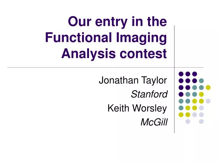
Our entry in the Functional Imaging Analysis contest Jonathan Taylor Stanford Keith Worsley McGill
What is functional Magnetic Resonance Imaging (fMRI) data? • Time series of ~200 “frames”, 3D images of brain “activity”, taken every ~2.5s (~8min) • Meanwhile, subject receives stimulus or external task (e.g on/off every 10s) • Several (~4) time series (“runs”) per session • Several (~2) sessions per subject • Several (~15) subjects • Statistics problem: find the regions of the brain activated by the stimulus or task
Why a Functional Imaging Analysis Contest (FIAC)? • Competing packages produce slightly different results, which is “correct”? • Simulated data? • Real data, compare analyses • “Contest” session at 2005 Human Brain Map conference • 9 entrants • Results in a special issue of Human Brain Mapping in May, 2006
The main participants • SPM (Statistical Parametric Mapping, 1993), University College, London, “SAS”, (MATLAB) • AFNI (1995), NIH, more display and manipulation, not much stats (C) • FSL (2000), Oxford, the “upstart” (C) • …. • FMRISTAT (2001), McGill, stats only (MATLAB) • BRAINSTAT (2005), Stanford/McGill, Python version of FMRISTAT
Alternating hot and warm stimuli separated by rest (9 seconds each). 2 warm warm hot hot 1 0 -1 0 50 100 150 200 250 300 350 Hemodynamic response function: difference of two gamma densities 0.4 0.2 0 -0.2 0 50 Responses = stimuli * HRF, sampled every 3 seconds 2 1 0 -1 0 50 100 150 200 250 300 350 Time, seconds Effect of stimulus on brain response • Modeled by convolving the stimulus with the “hemodynamic response function” Stimulus is delayed and dispersed by ~6s
First scan of fMRI data Highly significant effect, T=6.59 1000 hot 890 rest 880 870 warm 500 0 100 200 300 No significant effect, T=-0.74 820 hot 0 rest 800 T statistic for hot - warm effect warm 5 0 100 200 300 Drift 810 0 800 790 -5 0 100 200 300 Time, seconds fMRI data, pain experiment, one slice T = (hot – warm effect) / S.d. ~ t110 if no effect
How fMRI differs from other repeated measures data • Many reps (~200 time points) • Few subjects (~15) • Df within subjects is high, so not worth pooling sd across subjects • Df between subjects low, so use spatial smoothing to boost df • Data sets are huge ~4GB, not easy to use R directly
FMRISTAT / BRAINSTATstatistical analysis strategy • Analyse each voxel separately • Borrow strength from neighbours when needed • Break up analysis into stages • 1st level: analyse each time series separately • 2nd level: combine 1st level results over runs • 3rd level: combine 2nd level results over subjects • Cut corners: do a reasonable analysis in a reasonable time (or else no one will use it!) • MATLAB / Python
1st level: Linear model with AR(p) errors • Data • Yt = fMRI data at time t • xt = (responses,1, t, t2, t3, … )’ to allow for drift • Model • Yt = xt’β + εt • εt = a1εt-1 + … + apεt-p + σFηt, ηt ~ N(0,1) i.i.d. • Fit in 2 stages: • 1st pass: fit by least squares, find residuals, estimate AR parameters a1 … ap • 2nd pass: whiten data, re-fit by least squares
Higher levels:Mixed effects model • Data • Ei = effect (contrast in β) from previous level • Si = sd of effect from previous level • zi = (1, treatment, group, gender, …)’ • Model • Ei = zi’γ + SiεiF + σRεiR (Si high df, soassumed fixed) • εiF ~ N(0,1) i.i.d. fixed effects error • εiR ~ N(0,1) i.i.d. random effects error • Fit by ReML • Use EM for stability, 10 iterations
Where we use spatial information • 1st level: smooth AR parameters to lower variability and increase “df” • Higher levels: smooth Random / Fixed effects sd ratio to lower variability and increase “df” • Final level: use random field theory to correct for multiple comparisons
1st level: Autocorrelation AR(1) model: εt = a1εt-1 + σFηt • Fit the linear model using least squares • εt = Yt – Yt • â1 = Correlation (εt , εt-1) • Estimating errort’schanges their correlation structure slightly, so â1 is slightly biased: • Raw autocorrelation Smoothed 12.4mm Bias corrected â1 ~ -0.05 ~ 0
How much smoothing? • Variability in acor lowers df • Df depends • on contrast • Smoothing acor brings df back up: dfacor = dfresidual(2 + 1) 1 1 2 acor(contrast of data)2 dfeffdfresidualdfacor FWHMacor2 3/2 FWHMdata2 = + Hot-warm stimulus Hot stimulus FWHMdata = 8.79 Residual df = 110 Residual df = 110 100 100 Target = 100 df Target = 100 df Contrast of data, acor = 0.79 50 Contrast of data, acor = 0.61 50 dfeff dfeff 0 0 0 10 20 30 0 10 20 30 FWHM = 10.3mm FWHM = 12.4mm FWHMacor FWHMacor
Higher order AR model? Try AR(3): No correlation biases T up ~12% → more false positives a a a 1 2 3 0.3 0.2 AR(1) seems to be adequate 0.1 0 … has little effect on the T statistics: -0.1 AR(1), df=100 AR(2), df=99 AR(3), df=98 5 0 -5
Run 1 Run 2 Run 3 Run 4 2nd level 1 Effect, 0 E i -1 0.2 Sd, S 0.1 i 0 5 T stat, 0 E / S i i -5 2nd level: 4 runs, 3 df for random effects sd … very noisy sd: … and T>15.96 for P<0.05 (corrected): … so no response is detected …
Solution: Spatial smoothing of the sd ratio • Basic idea: increase df by spatial smoothing (local pooling) of the sd. • Can’t smooth the random effects sd directly, - too much anatomical structure. • Instead, • random effects sd • fixed effects sd • which removes the anatomical structure before smoothing. ) sd= smooth fixed effects sd
^ Average Si Random effects sd, 3 df Fixed effects sd, 440 df Mixed effects sd, ~100 df 0.2 0.15 0.1 0.05 0 divide multiply Smoothed sd ratio Random sd / fixed sd 1.5 random effect, sd ratio ~1.3 1 0.5
400 300 200 100 0 0 20 40 Infinity How much smoothing? FWHMratio2 3/2 FWHMdata2 dfrandom = 3, dffixed = 4 110 = 440, FWHMdata = 8mm: dfratio = dfrandom(2 + 1) 1 1 1 dfeffdfratiodffixed = + fixed effects analysis, dfeff = 440 dfeff FWHM = 19mm Target = 100 df random effects analysis, dfeff = 3 FWHMratio
Run 1 Run 2 Run 3 Run 4 2nd level 1 Effect, 0 E i -1 0.2 Sd, S 0.1 i 0 5 T stat, 0 E / S i i -5 Final result: 19mm smoothing, 100 df … less noisy sd: … and T>4.93 for P<0.05 (corrected): … and now we can detect a response!
Final level: Multiple comparisons correction Bonferroni 4.7 4.6 4.5 True T, 10 df 4.4 Random Field Theory 4.3 T, 20 df Gaussianized threshold Discrete Local Maxima (DLM) 4.2 4.1 Gaussian 4 3.9 3.8 3.7 0 1 2 3 4 5 6 7 8 9 10 FWHM of smoothing kernel (voxels) Low FWHM: use Bonferroni In between: use Discrete Local Maxima (DLM) High FWHM: use Random Field Theory
0.12 Gaussian T, 20 df T, 10 df 0.1 Random Field Theory Bonferroni 0.08 0.06 P-value 0.04 Discrete Local Maxima True DLM can ½ P-value when FWHM ~3 voxels 0.02 0 0 1 2 3 4 5 6 7 8 9 10 FWHM of smoothing kernel (voxels) Low FWHM: use Bonferroni In between: use Discrete Local Maxima (DLM) High FWHM: use Random Field Theory
FIAC paradigm • 16 subjects • 4 runs per subject • 2 runs: event design • 2 runs: block design • 4 conditions per run • Same sentence, same speaker • Same sentence, different speaker • Different sentence, same speaker • Different sentence, different speaker • 3T, 191 frames, TR=2.5s
Response • Events • Blocks Beginning of block/run
Design matrix for block expt • B1, B2 are basis functions for magnitude and delay:
1st level analysis • Motion and slice time correction (using FSL) • 5 conditions • Smoothing of temporal autocorrelation to control the effective df
Efficiency • Sd of contrasts (lower is better) for a single run, assuming additivity of responses • For the magnitudes, event and block have similar efficiency • For the delays, event is much better.
2nd level analysis • Analyse events and blocks separately • Register contrasts to Talairach (using FSL) • Bad registration on 2 subjects - dropped • Combine 2 runs using fixed FX • Combine remaining 14 subjects using random FX • 3 contrasts × event/block × magnitude/delay = 12 • Threshold using best of Bonferroni, random field theory, and discrete local maxima (new!) 3rd level analysis
Part of slice z = -2 mm
Event Block Magnitude Delay
Events vs blocks for delaysin different – same sentence • Events: 0.14±0.04s; Blocks: 1.19±0.23s • Both significant, P<0.05 (corrected) (!?!) • Answer: take a look at blocks: Greater magnitude Different sentence (sustained interest) Best fitting block Same sentence (lose interest) Greater delay
Magnitude increase for • Sentence, Event • Sentence, Block • Sentence, Combined • Speaker, Combined at (-54,-14,-2)
Magnitude decrease for • Sentence, Block • Sentence, Combined at (-54,-54,40)
Delay increase for • Sentence, Event at (58,-18,2) inside the region where all conditions are activated
Conclusions • Greater %BOLD response for • different – same sentences (1.08±0.16%) • different – same speaker (0.47±0.0.8%) • Greater latency for • different – same sentences (0.148±0.035 secs)
z=-12 z=2 z=5 1 2 3 1,4 3 3 3 3 1 The main effects of sentence repetition (in red) and of speaker repetition (in blue).1: Meriaux et al, Madic; 2: Goebel et al, Brain voyager; 3: Beckman et al, FSL; 4: Dehaene-Lambertz et al, SPM2. Brainstat: combined block and event, threshold at T>5.67, P<0.05.
0.6 0.4 0.2 0 -0.2 -0.4 -5 0 5 10 15 20 25 t (seconds) Estimating the delay of the response • Delay or latency to the peak of the HRF is approximated by a linear combination of two optimally chosen basis functions: delay basis1 basis2 HRF shift • HRF(t + shift) ~ basis1(t)w1(shift) + basis2(t)w2(shift) • Convolve bases with the stimulus, then add to the linear model
3 2 1 0 -1 -2 -3 -5 0 5 shift (seconds) • Fit linear model, • estimate w1andw2 • Equate w2/w1to estimates, then solve for shift (Hensen et al., 2002) • To reduce bias when the magnitude is small, use • shift / (1 + 1/T2) • where T = w1/ Sd(w1) is the T statistic for the magnitude • Shrinks shift to 0 where there is little evidence for a response. w2 /w1 w1 w2
Magnitude (%BOLD), stimulus average Subject id, event experiment Mixed 0 1 3 4 6 7 8 9 10 11 12 13 14 15 effects 6 4 Ef 2 0 Random /fixed -2 effects sd smoothed Contour is: average anatomy > 2000 10.836mm 2 1.5 1.5 Sd 1 1 0.5 0 0.5 df 200 200 200 200 200 100 200 200 200 200 200 200 200 200 100 FWHM (mm) 20 20 50 5 15 15 100 x (mm) T 10 10 150 0 5 5 200 250 -5 0 0 120 140 160 180 P=0.05 threshold for peaks is +/- 5.1687 y (mm)
Magnitude (%BOLD), stimulus average Subject id, block experiment Mixed 0 1 3 4 6 7 8 9 10 11 12 13 14 15 effects 4 Ef 2 Random 0 /fixed effects sd smoothed Contour is: average anatomy > 2000 6.7765mm 1 6 Sd 0.5 4 2 0 df 209 209 214 210 211 210 210 207 212 214 214 210 210 216 99 FWHM (mm) 20 20 20 -50 15 15 15 10 x (mm) T 0 10 10 5 5 5 0 50 -5 0 0 -60 -40 -20 0 P=0.05 threshold for peaks is +/- 5.9873 y (mm)
Magnitude (%BOLD), diff - same speaker Subject id, event experiment Mixed 0 1 3 4 6 7 8 9 10 11 12 13 14 15 effects 2 1 Ef 0 -1 Random /fixed -2 effects sd smoothed Contour is: average anatomy > 2000 11.7848mm 2 1.5 1.5 Sd 1 1 0.5 0 0.5 df 273 271 276 281 274 136 265 293 264 268 265 264 296 270 100 FWHM (mm) 5 20 20 -50 15 15 x (mm) T 0 0 10 10 5 5 50 -5 0 0 -60 -40 -20 0 P=0.05 threshold for peaks is +/- 5.1469 y (mm)
Magnitude (%BOLD), diff - same speaker Subject id, block experiment Mixed 0 1 3 4 6 7 8 9 10 11 12 13 14 15 effects 2 1 Ef 0 -1 Random /fixed -2 effects sd smoothed Contour is: average anatomy > 2000 11.9735mm 1 1.5 Sd 0.5 1 0 0.5 df 201 202 200 206 201 201 200 200 204 204 206 201 205 204 100 FWHM (mm) 5 20 20 -50 15 15 x (mm) T 0 0 10 10 5 5 50 -5 0 0 -60 -40 -20 0 P=0.05 threshold for peaks is +/- 5.1666 y (mm)
Magnitude (%BOLD), interaction Subject id, event experiment Mixed 0 1 3 4 6 7 8 9 10 11 12 13 14 15 effects 2 1 Ef 0 -1 Random /fixed -2 effects sd smoothed Contour is: average anatomy > 2000 11.4737mm 2 1.5 1.5 Sd 1 1 0.5 0 0.5 df 278 278 279 280 264 126 277 287 264 272 260 277 264 264 100 FWHM (mm) 5 20 20 -50 15 15 x (mm) T 0 0 10 10 5 5 50 -5 0 0 -60 -40 -20 0 P=0.05 threshold for peaks is +/- 5.4124 y (mm)
Magnitude (%BOLD), interaction Subject id, block experiment Mixed 0 1 3 4 6 7 8 9 10 11 12 13 14 15 effects 2 1 Ef 0 -1 Random /fixed -2 effects sd smoothed Contour is: average anatomy > 2000 12.1993mm 1 1.5 Sd 0.5 1 0 0.5 df 204 200 207 200 204 205 202 203 202 204 206 201 201 200 100 FWHM (mm) 5 20 20 -50 15 15 x (mm) T 0 0 10 10 5 5 50 -5 0 0 -60 -40 -20 0 P=0.05 threshold for peaks is +/- 5.1467 y (mm)