Download
1 / 26
290 likes | 690 Views
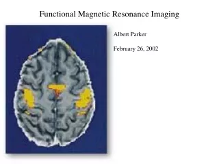
Functional magnetic resonance imaging. Magnetic resonance imaging. My discussion: MRI procedure. generate tissue contrast generate spatial localization. larmor frequency and RF pulse. Larmor frequency. RF pulse(classical view). z. B 0. M. . y. x’. y’. x. . Tissue contrast. y.

E N D
My discussion: MRI procedure • generate tissue contrast • generate spatial localization
larmor frequency and RF pulse • Larmor frequency • RF pulse(classical view) z B0 M y x’ y’ x
y y x x z z intrinsic spin-spin interactions T2 decay constant B’ 90o RF(B1) pause removed Classical viewpoint Mxy Mxy
Spin-lattice relaxation T1 relaxation constant 90o RF(B1) pause added energy
Spin-echo 180o 180o 90o 90o RF signal T2* T2 TE TR T2=spin-spin relaxation T2*=T2+static field inhomogeneities
Different contrast images T2 contrast : TR/TE = 5500/105 ms, 2 Nex, 512x256 matrix White Grey CSF TE(14) TR(450) TR(5500) TE(105) T1 contrast : TR/TE= 450/14 ms, 1 Nex, 256x192 matrix *Nex: number of acquisitions
Spatial localization • Slice select gradient • Frequency encode gradient • Phase encode gradient
Slice select gradient: slice thickness 2 ’ RF bandwidth B+ 2 0 B0 B- D1 Z D2 D3
Slice select gradient: slice location B+ RF bandwidth 2 0 B0 B- Z2 Z1 Z3 Z
Frequency encode gradient +Bx -Bx digitization +f max -f max 0 Fourier transform
Phase encode gradient #128 #188 #60 - + Time #256 #1 - + - + - +
y x f(x,y) repeat Imaging: spin echo 90o 180o RF pause Slice selection gradient Phase encode gradient Frequency encode gradient ky MR signal kx Data acquisition F(kx,ky) MR image k-space
90o 180o Imaging: spin echo planar-FMRI technique repeat RF pause Slice selection gradient Phase encode gradient Within T2* Frequency encode gradient MR signal Data acquisition ky y kx x F(kx,ky) f(x,y) MR image k-space
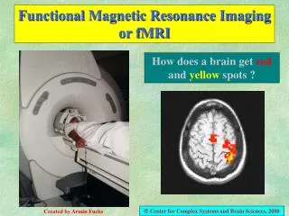
Functional magnetic resonance imaging • BOLD(blood-oxygen-level-dependent) fMRI is currently the most common fMRI technique • Noninvasive-no injection of radioactive isotopes • Spin echo planar imaging-extremely fast-50 ms • T2-T2* weighted images
T2-T2* weighted image: T2* is dependent on the presence of blood deoxygenation and that deoxygenated hemoglobin is a"BOLD" effect that can be observed by FMRI at high magnetic fields more paramagnetic shorter T2* longer T2*
FMRI images a high resolution scan is taken as background a series of low resolution scans are taken over time during the experiment the analyzed low resolution images are shown as colored blobs on top of the original high resolution scan, and also in 3D after proper analysis
The posterior lateral prefrontal cortex is a key neural substrate underlying the central bottleneck of information processing.
Central bottleneck model: Task 1 Task 2 Experimental result:
Advantage: • FMRI can precisely locate the brain active spot with 1.5 x 1.5 mm in-plane resolution or even less than 1 mm. • FMRI can catch the blood flow in seconds with total scan time on the order of 1.5 to 2.0 min per run.