Download
1 / 26
260 likes | 339 Views
Limited Area Models. Adam Sobel Banff Summer School. What do we mean by a limited area model?. A model whose domain is a subset of the entire global atmosphere. Usually this is done because higher resolution is desired, increasing the computational

E N D
Limited Area Models Adam Sobel Banff Summer School
What do we mean by a limited area model? A model whose domain is a subset of the entire global atmosphere. Usually this is done because higher resolution is desired, increasing the computational expense, so reducing the domain size compensates.
Generic issues • The boundaries of limited area models are artificial. In general there is no rigorous, well-posed way to formulate the boundary conditions (except idealized, e.g. periodic). This becomes more important for longer simulations, i.e. Regional Climate Models. • We go to higher resolution to reduce parameterization issues. Yet these can in some respects become worse as resolution increases. While some processes don’t need to be parameterized any more, others still do, and the parameterizations may become less justified as sample size of parameterized entities (clouds, turbulent eddies, etc.) in each grid box is reduced. • Because parameterizations must change as resolution does, there can be no convergence, in the standard sense, in full-physics atmospheric modeling.
Comprehensive models, what they parameterize, and what they’re good for. • General Circulation Models (GCMs). Cover the whole globe. Grid spacing typically O(200 km) in horizontal, 10+ levels in vertical. Hydrostatic. Lots of physics must be parameterized. Used for global weather (including your daily forecast) and climate. • Mesoscale/regional climate models. Cover finite part of globe. Grid spacing ~10-100 km. Nowadays usually nonhydrostatic (but often not fully compressible). Same # of parameterizations as GCMs, but sometimes different ones, esp. for convection. Used for study of individual synoptic-scale weather events, and regional climate prediction (downscaling).
Full physics models cont. • “Cloud Resolving” or Cumulus Ensemble Models. Grid spacing O(1 km). Nonhydrostatic. Convection isn’t parameterized. PBL maybe, maybe not. Used for study of individual mesoscale weather events, and testing of parameterizations for larger-scale models. • “Large Eddy Simulation” (LES). A misnomer! Grid spacing ~10-100 m. Usually used for studies of PBL. The “energy-containing” eddies in what was considered small-scale turbulence (in CRM for example) are resolved, but lower inertial/dissipation range isn’t. Still need to parameterize radiation, microphysics, and the really small-scale turbulence. • Direct numerical simulation. Grid spacing at the Kolmogorov microscale (~mm-cm). No parameterizations. Not practical for too many problems of interest.
Mesoscale/regional climate models • Roughly like GCMs in physics/dynamics partitioning (unless run at CRM resolution, in which case conv. scheme turned off) • Grids can be and often are nested. • Mesoscale model: Nonhydrostatic. Used mainly for weather simulations (~few days). Initial conditions are important. • Regional climate model: Usually hydrostatic. Longer-term simulations, e.g. for “downscaling” of global climate predictions. BCs dominate - and are not necessarily well-posed! Come from GCM, or from assimilation data set (e.g. Reanalyses) – RCM “nudged” towards forcing data at boundaries. Usually one-way nesting.
Example 1: Case study of a weather event using a mesoscale model California “pineapple express” flood 1996-97, Penn State/NCAR MM5 model, figure courtesy Joe Galewsky. (Galewsky & Sobel, MWR, in press, avail. at www.columbia.edu/~ahs129/home.html) near-surface e and precip
Example 2: your short-term weather forecasts NCEP “Eta” model, 500 hPa forecast issued 5/2/2005. Global models are now also run at similar resolution, erasing GCM-mesoscale distinction.
Example 3: A regional climate simulation Regional climate (and GCM) simulation of tropical Atlantic rainfall for April 1994, courtesy Deborah Herceg. RCM domain is shown. Simulation run for 1 month.
Mesoscale/regional climate modeling issues • Boundary conditions – not well posed to begin with. More than one way of formulating them. Matters more for RCM. • This leads to sensitivity to domain choice. Don’t put boundaries near anything important. • At 10-100 km horizontal grid spacing, basis for convective parameterization becomes questionable, as mesoscale systems start to be resolved.
Cloud resolving models • horizontal grid size ~0.5-5 km • no convective parameterization • boundary layer parameterization maybe, maybe not – now basis for this becomes questionable as largest PBL eddies are close to being resolved • cloud microphysics, radiation, subgrid-scale turbulence parameterized • boundary conditions can be “open”, for short-term weather simulations, or periodic, for use like an RCM • In the latter case, large-scale “forcings” may be applied, as in parameterization testing mode of RCM • Sometimes run in 2D, which brings up additional issues
Short-term simulations usually used to understand dynamics of mesoscale cloud systems Radar data; Houze et al., Bull. Amer. Meteor. Soc., 1989
3D CRM Simulation of mesoscale system cloud (white) & precipitation water (yellow) Courtesy W.-K. Tao, NASA Goddard Mesoscale group
CRMs in SCM mode • E.g., for testing convective parameterizations, by getting realizations of distributed fields for same forcings • Forced same way as SCM – with large-scale advective terms. These do not appear in the mass budget (though they should). • For forcings=0, get Radiative-convective equilibrium • Generally periodic BCs, to allow long simulations – primary interest is often in statistics, rather than details of individual systems
Cloud-resolving simulation RCE, aim to understand spontaneous convective organization (Tompkins 2001, J. Atmos. Sci.58, 1650–1672)
Same forcing issues as with SCMs • For long-term tropical simulations with prescribed advective forcings, vertical advection term more or less determines precipitation • Still many things meaningfully simulated (T & q, cloud structure, radiative interactions…) • For determining large-scale controls in precip by e.g., SST, can use weak temperature gradient approach
WTG CRM simulation (Perez et al., manuscript submitted to JAS) • Goddard Cumulus Ensemble Model • 2D – so mean horizontal wind strongly nudged • No mean shear • No horizontal advection terms (incl. moisture) • WTG – strongly relax free-tropospheric T towards prescribed profile (taken from RCE simulation) – is then implied as that necessary so s/p = Q; that then used in moisture equation • Vary SST, keeping all else, including T(p) above PBL, fixed MS available at www.columbia.edu/~ahs129/pubs.html
SST vs. Precip Dashed lines are SST & P of the RCE used to derive T(p) Right or wrong, the result at least depends nontrivially on model physics.
Large-Eddy Simulation • Really about simulating small eddies – resolution in 5-100 m range • Mainly used for studying PBL turbulence • “Large” eddies means “energy-containing” in the sense of Kolmogorov – grid size should capture at least some of the inertial range • Subgrid-scale (hopefully dissipation-range) eddies still parameterized, so this is not Direct Numerical Simulation • If cloud microphysics & radiation included, must parameterize them
Entrainment across the inversion capping a convective BL Potential temperature contours delineate the inversion Sullivan et al. 1998, JAS,55, pp. 3042–3064
Recent developments en route to global CRMs. • “Super–Parameterization” (Grabowski, Randall, Arakawa, Khairoutdinov): put CRM on subset of GCM grid box, in lieu of parameterization • “DARE/RAVE” (Kuang, Blossey, Bretherton, Pauluis): run global (or near-global CRM) but reduce computational cost by reducing the time and length scales of the “large-scale” flow
Initial attempts at Super-Parameterization: MJO Original T21 GCM GCM with Super-Param Randall et al. 2003: BAMS84, 1547–1564.
DARE • “Diabatic Acceleration and Rescaling” (Kuang et al. 2005, Geophys. Res. Lett., 32, L02809, doi: 10.1029/2004GL021024.) • Reduce size of planet by factor ; increase rotation rate by ; also speed up all diabatic processes (surface & radiative fluxes, microphysical timescales etc.) by . Gives a planet in which large-scale and convective scale are not as widely separated. • Same effect can be obtained by just reducing g (Pauluis, Held).
Self-aggregation and sensitivity to domain size in RCE Bretherton et al,. An energy-balance analysis of deep convective self-aggregation above uniform SST, JAS, in press Day 50 Day 6 Only happens for domains ≥ 400x400 km!