Download
1 / 46
470 likes | 591 Views
Data Modeling General Linear Model & Statistical Inference. Thomas Nichols, Ph.D. Assistant Professor Department of Biostatistics http://www.sph.umich.edu/~nichols Brain Function and fMRI ISMRM Educational Course July 11, 2002. Motivations. Data Modeling Characterize Signal

E N D
Data ModelingGeneral Linear Model &Statistical Inference Thomas Nichols, Ph.D. Assistant Professor Department of Biostatistics http://www.sph.umich.edu/~nichols Brain Function and fMRI ISMRM Educational Course July 11, 2002
Motivations • Data Modeling • Characterize Signal • Characterize Noise • Statistical Inference • Detect signal • Localization (Where’s the blob?)
Outline • Data Modeling • General Linear Model • Linear Model Predictors • Temporal Autocorrelation • Random Effects Models • Statistical Inference • Statistic Images & Hypothesis Testing • Multiple Testing Problem
Basic fMRI Example • Data at one voxel • Rest vs.passive word listening • Is there an effect?
A Linear Model • “Linear” in parameters 1&2 error = + + b1 b2 Time e x1 x2 Intensity
Linear model, in image form… Estimated = + +
… in image matrix form… = +
= + Y … in matrix form. N: Number of scans, p: Number of regressors
Linear Model Predictors • Signal Predictors • Block designs • Event-related responses • Nuisance Predictors • Drift • Regression parameters
Signal Predictors • Linear Time-Invariant system • LTI specified solely by • Stimulus function ofexperiment • Hemodynamic ResponseFunction (HRF) • Response to instantaneousimpulse Blocks Events
Block Design Event-Related Convolution Examples Experimental Stimulus Function Hemodynamic Response Function Predicted Response
SPM’s HRF HRF Models • Canonical HRF • Most sensitive if it is correct • If wrong, leads to bias and/or poor fit • E.g. True responsemay be faster/slower • E.g. True response may have smaller/bigger undershoot
HRF Models • Smooth Basis HRFs • More flexible • Less interpretable • No one parameter explains the response • Less sensitive relativeto canonical (only if canonical is correct) Gamma Basis Fourier Basis
HRF Models • Deconvolution • Most flexible • Allows any shape • Even bizarre, non-sensical ones • Least sensitive relativeto canonical (again, ifcanonical is correct) Deconvolution Basis
Drift Models • Drift • Slowly varying • Nuisance variability • Models • Linear, quadratic • Discrete Cosine Transform Discrete Cosine Transform Basis
General Linear ModelRecap • Fits data Y as linear combination of predictor columns of X • Very “General” • Correlation, ANOVA, ANCOVA, … • Only as good as your X matrix
Temporal Autocorrelation • Standard statistical methods assume independent errors • Error i tells you nothing about j i j • fMRI errors not independent • Autocorrelation due to • Physiological effects • Scanner instability
Temporal AutocorrelationIn Brief • Independence • Precoloring • Prewhitening
Autocorrelation: Independence Model • Ignore autocorrelation • Leads to • Under-estimation of variance • Over-estimation of significance • Too many false positives
Autocorrelation:Precoloring • Temporally blur, smooth your data • This induces more dependence! • But we exactly know the form of the dependence induced • Assume that intrinsic autocorrelation is negligible relative to smoothing • Then we know autocorrelation exactly • Correct GLM inferences based on “known” autocorrelation [Friston, et al., “To smooth or not to smooth…” NI 12:196-208 2000]
Autocorrelation:Prewhitening • Statistically optimal solution • If know true autocorrelation exactly, canundo the dependence • De-correlate your data, your model • Then proceed as with independent data • Problem is obtaining accurate estimates of autocorrelation • Some sort of regularization is required • Spatial smoothing of some sort
Autocorrelation: Models • Autoregressive • Error is fraction of previous error plus “new” error • AR(1): i = i-1 + I • Software: fmristat, SPM99 • AR + White Noise or ARMA(1,1) • AR plus an independent WN series • Software: SPM2 • Arbitrary autocorrelation function • k = corr( i, i-k ) • Software: FSL’s FEAT
Statistic Images &Hypothesis Testing • For each voxel • Fit GLM, estimate betas • Write b for estimate of • But usually not interested in all betas • Recall is a length-p vector
Building Statistic Images Predictor of interest b1 b2 b3 b4 b5 b6 b7 b8 b9 = + ´ = + Y X b e
c’ = 1 0 0 0 0 0 0 0 b1b2b3b4b5.... contrast ofestimatedparameters c’b T = T = varianceestimate s2c’(X’X)+c Building Statistic Images • Contrast • A linear combination of parameters • c’
Hypothesis Test • So now have a value T for our statistic • How big is big • Is T=2 big? T=20?
P-val Hypothesis Testing • Assume Null Hypothesis of no signal • Given that there is nosignal, how likely is our measured T? • P-value measures this • Probability of obtaining Tas large or larger • level • Acceptable false positive rate T
Random Effects Models • GLM has only one source of randomness • Residual error • But people are another source of error • Everyone activates somewhat differently…
Distribution of each subject’s effect Fixed vs.RandomEffects Subj. 1 Subj. 2 • Fixed Effects • Intra-subject variation suggests all these subjects different from zero • Random Effects • Intersubject variation suggests population not very different from zero Subj. 3 Subj. 4 Subj. 5 Subj. 6 0
Random Effects for fMRI • Summary Statistic Approach • Easy • Create contrast images for each subject • Analyze contrast images with one-sample t • Limited • Only allows one scan per subject • Assumes balanced designs and homogeneous meas. error. • Full Mixed Effects Analysis • Hard • Requires iterative fitting • REML to estimate inter- and intra subject variance • SPM2 & FSL implement this, very differently • Very flexible
Random Effects for fMRIRandom vs. Fixed • Fixed isn’t “wrong”, just usually isn’t of interest • If it is sufficient to say “I can see this effect in this cohort”then fixed effects are OK • If need to say “If I were to sample a new cohort from the population I would get the same result”then random effects are needed
t > 2.5 t > 4.5 t > 0.5 t > 1.5 t > 3.5 t > 5.5 t > 6.5 Multiple Testing Problem • Inference on statistic images • Fit GLM at each voxel • Create statistic images of effect • Which of 100,000 voxels are significant? • =0.05 5,000 false positives!
MCP Solutions:Measuring False Positives • Familywise Error Rate (FWER) • Familywise Error • Existence of one or more false positives • FWER is probability of familywise error • False Discovery Rate (FDR) • R voxels declared active, V falsely so • Observed false discovery rate: V/R • FDR = E(V/R)
FWER MCP Solutions • Bonferroni • Maximum Distribution Methods • Random Field Theory • Permutation
FWER MCP Solutions • Bonferroni • Maximum Distribution Methods • Random Field Theory • Permutation
FWER MCP Solutions: Controlling FWER w/ Max • FWER & distribution of maximum FWER = P(FWE) = P(One or more voxels u | Ho) = P(Max voxel u | Ho) • 100(1-)%ile of max distn controls FWER FWER = P(Max voxel u | Ho) u
FWER MCP Solutions:Random Field Theory • Euler Characteristic u • Topological Measure • #blobs - #holes • At high thresholds,just counts blobs • FWER = P(Max voxel u | Ho) = P(One or more blobs | Ho) P(u 1 | Ho) E(u| Ho) Threshold Random Field Suprathreshold Sets
5% Parametric Null Max Distribution 5% Nonparametric Null Max Distribution Controlling FWER: Permutation Test • Parametric methods • Assume distribution ofmax statistic under nullhypothesis • Nonparametric methods • Use data to find distribution of max statisticunder null hypothesis • Any max statistic!
Measuring False Positives • Familywise Error Rate (FWER) • Familywise Error • Existence of one or more false positives • FWER is probability of familywise error • False Discovery Rate (FDR) • R voxels declared active, V falsely so • Observed false discovery rate: V/R • FDR = E(V/R)
Signal Measuring False PositivesFWER vs FDR Noise Signal+Noise
11.3% 11.3% 12.5% 10.8% 11.5% 10.0% 10.7% 11.2% 10.2% 9.5% 6.7% 10.5% 12.2% 8.7% 10.4% 14.9% 9.3% 16.2% 13.8% 14.0% Control of Per Comparison Rate at 10% Percentage of Null Pixels that are False Positives Control of Familywise Error Rate at 10% FWE Occurrence of Familywise Error Control of False Discovery Rate at 10% Percentage of Activated Pixels that are False Positives
p(i) i/V q Controlling FDR:Benjamini & Hochberg • Select desired limit q on E(FDR) • Order p-values, p(1)p(2) ... p(V) • Let r be largest i such that • Reject all hypotheses corresponding top(1), ... , p(r). 1 p(i) p-value i/V q 0 0 1 i/V
Conclusions • Analyzing fMRI Data • Need linear regression basics • Lots of disk space, and time • Watch for MTP (no fishing!)
Thanks • Slide help • Stefan Keibel, Rik Henson, JB Poline, Andrew Holmes