Download
1 / 23
240 likes | 313 Views
RETURN, RISK AND EQUILIBRIUM. BY PROF. SANJAY SEHGAL DEPARTMENT OF FINANCIAL STUDIES UNIVERSITY OF DELHI SOUTH CAMPUS NEW DELHI-110021 PH.: 0091-11-24111552 Email: sanjayfin15@yahoo.co.in K2. PROMINENT INVESTMENT OBJECTIVES. Regular income Income on Income Capital appreciation

E N D
RETURN, RISK AND EQUILIBRIUM BY PROF. SANJAY SEHGAL DEPARTMENT OF FINANCIAL STUDIES UNIVERSITY OF DELHI SOUTH CAMPUS NEW DELHI-110021 PH.: 0091-11-24111552 Email: sanjayfin15@yahoo.co.in K2
PROMINENT INVESTMENT OBJECTIVES • Regular income • Income on Income • Capital appreciation • Safety of capital • Liquidity • Tax considerations
THE TWO PARAMETER FRAMEWORK Maximize Expected Utility E(U) = f(Return, Risk) Pre-conditions for the Two-parameter to work in financial markets • Historical distribution of returns exhibit normality • Investor utility functions are quadratic in nature, i.e. E(U) f(mean, variance)
EX-ANTE RETURN AND RISK ON SECURITY i Expected Return E(Ri) = PiOi Standard Deviation of return i = Pi[Oi - E(Ri) ]2 Variance of returns Var(Ri) = 2
AN EXAMPLE Economic Probability Outcome (%) . scenario Security 1 Security 2 Good 0.3 25 40 Average 0.5 20 10 Poor 0.2 15 - 10 E(R1) = .3 x 25 + .5 x 20 + .2 x 15 = 20.5% E(R2) = .3 x 40 + .5 x 10 + .2 x -10 = 15% 1 = [.3(25 - 20.5)2 + .5(20 - 20.5)2 + .2(15 - 20.5)2]1/2 = 3.5% 2 = [.3(40 - 15)2 + .5(10 - 15)2 + .2(-10 - 15)2]1/2 = 18% approx.
EX-POST RETURN ON SECURITY i One- period return P1 – P0 D1 R1 = ----------- + ---------- P0 P0 Capital Dividend gains Yield yield NOTE: 1. Ignoring dividend yield one can compute approximate one-period return as P1 – P0 R1 = ----------- P0 2. The square of the period returns can be used to estimate average returns.
CAPITALISATION CHANGES AND STOCK PRICES • Stock Dividends If a firm issues a stock dividend on n:m, then ex-stock dividend price = m/(n+m), where n = new share issued, m = old shares with shareholders. Example: A firm issues tock dividend of 2:3, The ex-stock dividend price = 3/5. • Rights Issues nP1 + mP2 The ex-rights price of a firm = --------------- n + m where n = rights shares, m is old shares, n = issue price, m = last cum-rights selling price Example: A firm offers a rights price is 2:3. The issue price is IOE, while the cum-rights selling price is 25 Euros. 2 x 10 + 3 x 25 95 Ex-rights price = -------------------- = ----- = 19 Euros 2 + 3 5
Ex-rights price 19 Rights adjustments factor = ------------------------------------- = ---- Last cum-rights selling price 30 • Stock Splits If a firm announces a stock split of n:m, ten ex-stock split price is n/m. Example: If stock split is 1:10, then ex-stock split price is 1/10.
MEASURING AVERAGE RETURNS Geometric average returns Using one-period gross returns, we estimate Ex-post GM returns RGM = [(1 + R1) (1 + R2) … (1 + RK)1/K] - 1 Arithmetic average returns Using one period net return we estimate Ex-post arithmetic average returns as w E(R) or AM = Ri/N i=1 Arithmetic average is preferred because • Easier to compute • It has more desirable mathematical properties • A better proxy for forward looking returns.
ESTIMATING EX-POST RETURN: AN ILLUSTRATION Months Monthly Return (1%) 1 6 2 2 3 4 E(Rt) = Ri/3 = 4% 6 + 2 + 4 • Ex-post return based on arithmetic mean = ------------- = 4% 3 2. Ex-post return base don geometric mean = cube root of [(1.06) (1.02) (1.04)] – 1 = [(1.06) (1.02) (1.04)]1/3 – 1 =
EX-POST MEASURES OF RISK Total risk measure standard deviation of returns i = 1/N-1 (Ri - E(Ri))2 An Example Months Monthly Return (1%) 1 6 2 2 3 4 E(Rt) = Ri/3 = 4% i = ½ [(6 - 4)2 + (2 - 4)2 + (4 - 4)2] = 2% NOTE: Standard deviation as a risk measure assumes that historical returns follow a normal distribution
DECOMPOSING TOTAL RISK Total Risk = systematic risk + unsystematic risk 2i = 2i 2M + 2ei Systematic risk variations in stock returns is owing to shifts in common macro-economic factors. Unsystematic risk: variation in stock returns is owing to micro-economic shocks. • Unsystematic risk is diversifiable in a large portfolio. • Sources of unsystematic risk • Industry factors • Group factors • Common factors • Firm specific factors.
BETA AS A MEASURE OF SYSTEMATIC RISK • Beta measures the sensitivity of stock returns to market index returns. • It is estimated as the slope of the regression of stock returns on market returns. Rit = α + β RMt + eit • Mathematically Cov RiRM β = ---------------- Var RM
STOCK CLASSIFICATION ON THE BASIS OF BETAS β > 1 Aggressive stocks β = 1 Average stocks β < 1 but > 0 Defensive stocks β = 0 Risk-free asset β < 0 Hedging stocks
BETA AND STOCK CLASSIFICATION Estimating Beta of a listed company - An Example Problem Month Return on Return on security i (%) Market Index 1 10 12 2 6 5 3 13 18 4 -4 -8 5 13 10 6 14 7 7 4 15 8 18 30 9 24 25 10 22 Solution Cov RiRM = .778 Var (RM) 1022 Cov RiRM I = ------------- = 0.76 Var RM
Time Series Regression: Estimating Beta for HDFC Bank stock Time Period: 2005-2007 Market Index : CNX S&P 500 The Model: Rit= a + bRmt Output: Rit = 0.142 + 0.704Rmt (1.126) (3.393) R2= 0.313
Regression Results using Excel: Estimating Beta for HDFC Bank stock
PRECAUTIONS WHILE ESTIMATING BETA • Number of observations: 48 - 60 • Observation frequency: monthly or weekly data • Market index: broad-based and value-weighted • Trading frequency: Active trading record.
UNLEVERED AND LEVERED BETAS • Unlevered Beta is a measure of operating risk of the firm. • Levered Beta is a measure of both operating and as well as financial risk of the firm. βL = βU [1 + (1 – TC)] D/E Or βU = βL/[1 + (1 – TC)] D/E
THE RELATIONSHIP BETWEEN RISK AND RETURN Estimating required returns: THE CAPITAL ASSET PRICING MODEL or CAPM approach R(R) = RF + (ERM – RF) βi Estimating expected returns: DIVIDEND CAPITALISATION MODEL APPROACH D1 D1 P0 = ------------- or ER = ----- + g ER – g P0
AN EXAMPLE Risk-free rate of return = 10% Return on market index = 14% Beta of IBM stock = 1.25 Dividend paid last year by IBM = 1.70 E Growth rate of IBM = 6% Current price of IBM stock = 22E Estimating R(R) R(R) = 10 + (14 – 10) 1.25 = 15% Estimating E(R) 1.70 (1.06) E(R) = -------------- + .06 = 14.18% 22 Since, ER < RR, IBM stock is overvalued. This is a sell signal
Equilibrium Value of IBM stock D1 Eqn. P0 = ------------- R (R) – g 1.80 = ----------- = 20 E .15 - .06 Since P0 (22E) > Eqm. P0 (20E), the stock is overvalued. It is a sell signal.
CHANGE IN EQUILIBRIUM PRICE Change in response to changes in underlying variables. Variable Old Value Revised value RF 10% 9% ERM - RF 4% 3% 1.25 1.33 g 6% 8% Revised R(R) = 9 + 3 (1.33) = 13% 1.70 (1.08) Eqm Price = -------------- .13 - .08 = 36.80 E