Download
1 / 45
501 likes | 647 Views
Risk and Return. By Jairaj Gupta. Session Objective. At the end of this session you should: Be aware of the key measures of risk and return for individual stocks and for portfolios. Be familiar with the effects of diversification

E N D
Risk and Return By Jairaj Gupta
Session Objective At the end of this session you should: • Be aware of the key measures of risk and return for individual stocks and for portfolios. • Be familiar with the effects of diversification • Understand the distinction between total risk, diversifiable risk and non-diversifiable risk. • The effect of changing correlation between the assets on the standard deviation of a portfolio. • Understand what is the risk-return–efficient frontier of risky assets?
What is Risk? • In general we can say risk is the deviation from expected outcome. • Risk is often perceived negatively. • A risky asset is one for which the return that will be realized in the future is not known with certainty. • Thus risk includes not only bad outcomes but also good outcomes. • Thus risk is a mix of danger & opportunity • Risk may emerge due to macroeconomic fluctuations, changing fortunes of various industries, asset-specific unexpected developments etc.
Expected Return & Risk: Basic Ideas • The quantification of risk and return is a crucial aspect of modern finance. It is not possible to make “good” (i.e., value-maximizing) financial decisions unless one understands the relationship between risk and return. • Rational investors like returns and dislike risk. • The following proxies are helpful in analyzing return and risk: Expected return - weighted average of the distribution of possible returns in the future. Variance of returns - a measure of the dispersion of the distribution of possible returns in the future. How do we calculate these measures?
Scenario Analysis and Probability Distributions • When we attempt to quantify risk, we begin with the question: What HPRs are possible, and how likely are they? • Scenario Analysis is the process of devising a list of possible economic scenarios and specifying the likelihood of each one, as well as the HPR that will be realized in each case.
Scenario Analysis and Probability Distributions • Probability distribution is the list of possible outcomes with associated probabilities. • Expected return is the mean value of the distribution of possible future returns.
Scenario Analysis and Probability Distributions • Variance of returns is a measure of the dispersion of the distribution of possible returns in the future.
Expected Return & Variance: Example2 • II. Variances Var(RA) = 0.40 x (.30 - .06)2 + 0.60 x (-.10 - .06)2 = .0384 Var(RB) = 0.40 x (-.05 - .13)2 + 0.60 x (.25 - .13)2 = .0216 • III. Standard deviations
A Relative Measure of Risk In some cases, an unadjusted variance or standard deviation can be misleading. If conditions for two or more investment alternatives are not similar—that is, if there are major differences in the expected rates of return—it is necessary to use a measure of relative variability to indicate risk per unit of expected return. A widely used relative measure of risk is the coefficient of variation (CV), calculated as follows:
Expected Return & Variance: Example2 • CV(A) = 19.6/6 = 3.27 • CV(B) = 14.7/13 = 1.13 Hence being a rational investor we will select asset B as it’s risk per unit return is lower than asset A.
Problem • During the past five years, you owned two stocks that had the following annual rates of return: a. Compute the arithmetic mean annual rate of return for each stock. Which stock is most desirable by this measure? b. Compute the standard deviation of the annual rate of return for each stock. By this measure, which is the preferable stock? c. Compute the coefficient of variation for each stock. By this relative measure of risk, which stock is preferable?
Portfolio Expected Returns and Variances • What we have done so far is describe the risk and return of individual securities. We also want to be able to describe the risk and return of portfolios of securities. • Markowitz considered diversification and showed that it is possible to combine assets with returns that are less than perfectly positively correlated, in a portfolio in an effort to lower portfolio risk without sacrificing return.
Assumptions of Markowitz Model 1. Investors consider each investment alternative as being represented by a probability distribution of expected returns over some holding period. 2. Investors maximize one-period expected utility, and their utility curves demonstrate diminishing marginal utility of wealth. 3. Investors estimate the risk of the portfolio on the basis of the variability of expected returns. 4. Investors base decisions solely on expected return and risk, so their utility curves are a function of expected return and the expected variance (or standard deviation) of returns only. 5. For a given risk level, investors prefer higher returns to lower returns. Similarly, for a given level of expected return, investors prefer less risk to more risk.
Portfolio Expected Returns and Variances • We have two equivalent alternatives open to us. • Component- We can determine the return and risk of the portfolio by combining the returns and risks of the securities that make up the portfolio. • Security - We can treat the portfolio as just another security and calculate its return and risk as we have been doing. • Both of these approaches give the same answer but the first allows us to see how individual securities affect the return and risk of a portfolio.
Portfolio Expected Returns and Variances Portfolioweights: put 50% in Asset A and 50% in Asset B: State of the Probability Return Return Return oneconomy of state on A on B portfolio Boom 0.40 30% -5% 12.5% Bust 0.60 -10% 25% 7.5% 1.00
Portfolio Expected Returns and Variances Calculate expected returns: Security approach E(RP) = 0.40 x (.125) + 0.60 x (.075) = .095 = 9.5% Component approach E(RP) = .50 x E(RA) + .50 x E(RB) = 9.5% Calculate variance of portfolio: Security approach Var(RP) = 0.40 x (.125 - .095)2 + 0.60 x (.075 - .095)2 = .0006 Portfolio approach The sum of the variances is NOT the variance of the portfolio Var (RP) ≠.50 x Var(RA) + .50 x Var(RB)
Measuring E(R) of Portfolio Mean return of a portfolio containing i securities with mean return E( can be calculated using the following equation.
Measuring Portfolio Variance of Returns • is the standard deviation of the portfolio. • is the weight of individual assets in the portfolio. • is the variance of returns of the asset i. • the covariance between the rates of returns of assets I and j . • = A)B)p
Covariance and Correlation • The risk of a portfolio is comprised of the risk of the individual securities plus the correlation between them. • If there are two securities then the risk of the portfolio can be calculated from the variance of each security plus the correlation between them. An alternative measure to the correlation is the co-variation or covariance between two securities. Varp= X12Var1+X22Var2+2X1X2Cov12
Covariance and Correlation • If there are more than two securities then the risk of the portfolio can be estimated from the variance of each security plus a correlation (or covariance) for each possible pair of securities in the portfolio. • E.g. if there are three securities then there are three variances (one for each security) and three possible correlations [between security 1 and 2, between security 1 and 3, and between security 2 and 3].
Covariance and Correlation One way of thinking of the components is to visualise a matrix of securities. Each security must pair with each other. If the numbers are the same it is a variance, otherwise a covariance. e.g. if there are five securities we can think of:
COMPUTATION OF COVARIANCE OF RETURNS FOR COCA-COLAAND HOME DEPOT: 2001
COMPUTATION OF STANDARD DEVIATION OF RETURNS FOR COCA-COLA AND HOME DEPOT: 2001
Measuring Portfolio Variance of Returns For two assets the variance can be calculated using the following equation: Assuming weights of Coca-Cola and Home Depot 0.5 each in the portfolio we get:
The Effect of less than perfectly +Ve correlation on Portfolio Variance Stock A returns Portfolio returns:50% A and 50% B Stock B returns 0.05 0.04 0.03 0.02 0.01 0 -0.01 -0.02 -0.03 -0.04 -0.05 0.04 0.03 0.02 0.01 0 -0.01 -0.02 -0.03 0.05 0.04 0.03 0.02 0.01 0 -0.01 -0.02 -0.03
Time Patterns Of Returns For Two Assets With Perfect Negative Correlation
Standard Deviations of Annual Portfolio Returns ( 3) (2) Ratio of Portfolio (1) Average Standard Standard Deviation to Number of Stocks Deviation of Annual Standard Deviation in Portfolio Portfolio Returns(%) of a Single Stock 1 49.24 1.00 10 23.93 0.49 50 20.20 0.41 100 19.69 0.40 300 19.34 0.39 500 19.27 0.39 1,000 19.21 0.39 These figures are from Table 1 in Meir Statman, “How Many Stocks Make a Diversified Portfolio?” Journal of Financial and Quantitative Analysis 22 (September 1987), pp. 353–64. They were derived from E. J. Elton and M. J. Gruber, “Risk Reduction and Portfolio Size: An Analytic Solution,” Journal of Business 50 (October 1977), pp. 415–37.
DIVERSIFICATION AND PORTFOLIO RISK • The principle of diversification states that as the covariance between returns for assets that are combined in a portfolio decreases, so does the variance of the return for that portfolio. • The “magic” is due to the degree of correlation between the expected asset returns. • The good news: investors can maintain expected return and lower portfolio risk by combining assets with low correlation. • The bad news: very few assets have small to negative correlations with other assets. • The problem becomes one of searching among large numbers of assets in an effort to discover the portfolio with the minimum risk at a given level of expected return.
DIVERSIFICATION AND PORTFOLIO RISK Primarily there are two sources of risk firm-specific (unique) risk and market risk. The former can be alleviated through efficient diversification, while the later cannot be alleviated. n is the number of securities.
Market Risk Market risk, systematic risk or non-diversifiable risk is emerges due to unfavorable changes in general economic conditions, such as the business cycle, the inflation rate, interest rates, exchange rates, and so forth. Market risk factors are common to whole economy and remains even after diversification.
Firm-specific Risk The risk that can be eliminated by diversification is called unique risk, firm-specific risk, nonsystematic risk, or diversifiable risk. These Firm-specific factors are those that affect the firm without noticeably affecting other firms and hence should be diversified.
Alternative Measures of Risk • Variance, or standard deviation of expected returns- The idea is that the more disperse the expected returns, the greater the uncertainty of future returns. • Range of returns - It is assumed that a larger range of expected returns, from the lowest to the highest return, means greater uncertainty and risk regarding future expected returns. • Semi-variance - A measure that only considers deviations below the mean, as positive deviations are favorable while negative deviations are unfavorable.
Portfolio Theory Portfolio theory is concerned with the choice of an efficient combinations of assets which minimizes the variance of a portfolio for a given level of return. Example: Expected Return Standard Deviation Dande 18% 35% Leeds plc 15% 30% Handy 12% 25% A portfolio that is 33.3% invested in each of the three stocks will have an expected return of 15% and a s.d. of 17.48% assuming the correlation between them is zero.
Assumptions of Portfolio Theory • The return on an investment adequately summarizes the outcome of the investment; an investor visualizes a probability distribution of rates of return; • Investors' risk estimates are proportional to the variance of return they perceive for a security or a portfolio. • Investors are willing to base their decisions on just two parameters of the probability distribution function - the expected return and the variance of returns; • The investor exhibits risk aversion, so for a given expected return he/she prefers minimum risk.
Investment Opportunity Set It is the set of available portfolio risk-return combinations.
Efficient Frontier Graph representing a set of portfolios that maximizes expected return at each level of portfolio risk.
Optimal Portfolio The optimal portfolio is the portfolio on the efficient frontier that has the highest utility for a given investor. It lies at the point of tangency between the efficient frontier and the curve with the highest possible utility.
Minimum Variance Portfolio • The minimum variance portfolio is the particular combination of securities that will result in the least possible variance. • For a two-security minimum variance portfolio, the proportions invested in stocks A and B are:
PORTFOLIO RISK-RETURN PLOTS FOR DIFFERENT WEIGHTS WHEN ri,j = + 1.00;+0.50; 0.00; –0.50; –1.00
Essential Readings: Text book: Z. Bodie, A. Kane and A. J. Marcus, Essentials of Investments, Mc-Graw Hill, 2008. Chapter 5. F. Reilly and K. Brown, Investment Analysis and Portfolio Management, South Western, 2006. Chapter 7
to get a copy of this presentation visit www.jairajgupta.weebly.com by jairajgupta e-mail: jairajgupta@gmail.com mobile: (+91) 9007202650