Download
1 / 9
90 likes | 214 Views
LECTURE 04: BASIC STATISTICAL MODELING OF DIGITAL SIGNALS. Objectives: Definition of a Digital Signal Random Variables Probability Density Functions Means and Moments White Noise

E N D
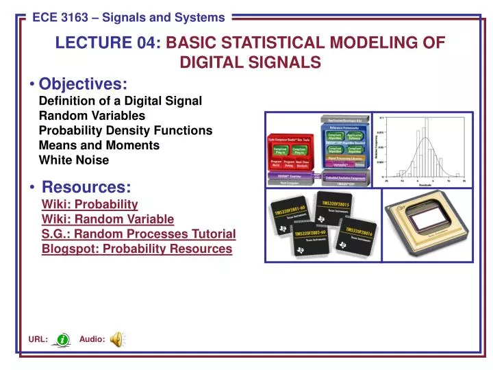
LECTURE 04: BASIC STATISTICAL MODELING OFDIGITAL SIGNALS • Objectives:Definition of a Digital SignalRandom VariablesProbability Density FunctionsMeans and MomentsWhite Noise • Resources:Wiki: ProbabilityWiki: Random VariableS.G.: Random Processes TutorialBlogspot: Probability Resources Audio: URL:
Introduction to Digital Signals • A discrete-time signal, x[n], is discrete in time but continuous in amplitude (e.g., the amplitude is represented as a real number). • We often approximate real numbers in digital electronics using a floating-point numeric representation (e.g., 4-byte IEEE floating-point numbers). • For example, a 4-byte floating point number uses 32 bits in its representation, which allows it to achieve 2**32 different values. • The simplest way to assign these values would be to use a linear representation: divide the range [Rmin,Rmax] into 2**32 equal steps. This is often referred to as linear quantization. Does this make sense? • Floating point numbers actually use a logarithmic representation consisting of an exponent and mantissa (e.g. IEEE floating-point format). • For many applications, such as encoding of audio and images, 32 bits per sample is overkill because humans can’t distinguish that many unique levels. • Lossless compression (e.g., gif images) techniques reduce the number of bits without introducing any distortion. • Lossy compression (e.g., jpeg or mp3) techniques reduce the number of bits significantly but introduce some amount of distortion. • Signals whose amplitude and time scale are discrete are referred to as digital signals and form the basis for the field of digital signal processing.
Signal Amplitude As A Random Variable • The amplitude of x[n] can be modeled as a random variable. Consider an audio signal (mp3-encoded music): • How would we compute a histogram of theamplitude of this signal? (Note that the exampleto the right is not an actual histogram of theabove data.) • What would be a reasonable approximation for the amplitude histogram of this signal? Frequency • Uniform Distribution • Triangular Distribution Amplitude • Gaussian Distribution -1.0 -0.5 0.0 0.5 1.0
Examples of Random Variables Continuous-valued random variable: Uniform: Triangular: Gaussian: Discrete-valued random variable: N/A • An important part of the specification of a random variable is its probability density function. Note that these integrate or sum to 1. • A Gaussian distribution is completely specified by two values, its mean and variance. This is one reason it is a popular and useful model. • Also note that quantization systems take into account the distribution of the data to optimize bit assignments. This is studied in disciplines such as communications and information theory.
Mean Value Of A Random Signal (DC Value) • The mean value of a random variable can be computed by integrating its probability density function: • Example: Uniformly Distributed Continuous Random Variable • The mean value of a discrete random variable can be computed in an analogous manner: • But this can also be computed using thesample mean (N = no. of samples): • In fact, in more advanced coursework, you will learn this is one of many ways to estimate the mean of a random variable (e.g., maximum likelihood). • For a discrete uniformly distributed random variable: • Soon we will learn that the average value of a signal is its DC value, or its frequency response at 0 Hz.
Variance and Standard Deviation • The variance of a continuous random variable can be computed as: • For a uniformly distributed random variable: • For a discrete random variable: • Following the analogy of a sample mean, this can be estimated from the data: • The standard deviation is just the square root of the variance. • Soon we will see that the variance is related to the correlation structure of the signal, the power of the signal, and the power spectral density.
Covariance and Correlation • We can define the covariance between two random variables as: • For time series, when y is simply a delayed version of x, this can be reduced to a simpler form known as the correlation of a signal: • For a discrete random variable representing the samples of a time series, we can estimate this directly from the signal as: • The correlation is often referred to as a second-order moment, with the expectation being the first-order moment. It is possible to define higher-order moments as well: • Two random variables are said to be uncorrelated if . • For a Gaussian random variable, only the mean and variance are non-zero; all other higher-order moments are equal to zero.
White Gaussian Noise • We can combine these concepts todevelop a model for noise. Consider asignal that has energy at all frequencies: • We can describe a signal like this ashaving a mean value of zero, a variance,or power, of 2. • It is common to model the amplitudedistribution of the signal as a Gaussiandistribution: • We refer to this as zero mean Gaussian white noise. • In many engineering systems corrupted by noise, we model the measured signal as: , where is zero-mean white Gaussian noise. • Why is this a useful model? Think about: • In Signals and Systems, continuous time, discrete-time and statistics converge to provide a powerful way to manipulate digital signals on a computer. This is one reason much instrumentation has gone digital.
Summary • Introduced the concept of a digital signal: a signal that is discrete in both time and amplitude. • Introduced the concept of a random variable, and showed how it can be modeled through a probability distribution of its value. We used this to model signals. • Introduced the concept of the mean and variance of a random variable. Demonstrated simple calculations of these for a uniformly distributed random variable. • Discussed the application of these to modeling noise. • MATLAB code for the examples discussed in this lecture can be found at: http://www.isip.piconepress.com/publications/courses/ece_3163/matlab/2009_spring/statistics. • Other similar signal processing examples are located at: http://www.isip.piconepress.com/publications/courses/ece_3163/matlab.