Download
1 / 16
170 likes | 391 Views
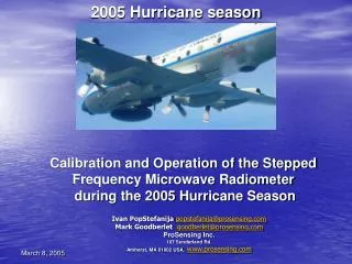
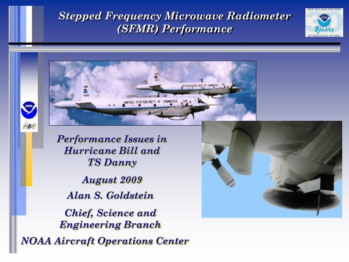
NOAA Aircraft Operations Center. Stepped Frequency Microwave Radiometer (SFMR) Performance. Performance Issues in Hurricane Bill and TS Danny August 2009. Alan S. Goldstein Chief, Science and Engineering Branch.

E N D
NOAA Aircraft Operations Center Stepped Frequency Microwave Radiometer(SFMR) Performance Performance Issues in Hurricane Bill and TS Danny August 2009 Alan S. Goldstein Chief, Science and Engineering Branch
One WP-3D (N43RF) participated in research missions for Hurricane Bill and Tropical Storm Danny. Flights occurred during the last two weeks of August 2009. • Surface wind data (generated from SFMR readings) received by the National Hurricane Center (NHC) had many missing data points, significantly worse than the historical performance of this instrument. • This report will show the underlying causes of the missing data and identify the partial solution that can be implemented in the short term.
After a series of vibration-related failures with AOC’s SFMR units, a loaner unit (S/N 18) was installed on N43RF. A calibration mission was flown on July 10, 2009. The data from that flight was provided to the SFMR manufacturer (ProSensing), who in turn calculated revised calibration constants to be used operationally. • AOC did an independent calculation of the revised constants, and verified that the ProSensing values were correct. • The plot below shows the modified constants provide errors within .5C across the range of unit (antenna) operating temperatures. Note that there is significant variation in the 6.02 GHz data.
Flight pattern on August 19, 2009 into Hurricane Bill. There were four eye penetrations. The course reversal near the start of the flight was when the C-band Scatterometer (C-Scatt) system failed. The mission continued with that system disabled.
Brightness temperatures for this flight. • Plots for Tb0-2 and Tb4 are (for the most part) hidden behind Tb5 plot, as would be expected • Note that Tb3 (6.02 GHz) is reading low, especially after 2:25Z, which is when aircraft ascended for return to base. This shows a problem with the offset and temperature correction values in the calibration table.
Expanded view of brightness temperatures as the aircraft arrived at operational altitude after initial ferry. • Dips in Tb’s are when the aircraft was in a roll. • Note that Tb3 had a significant offset until the first roll, then a small offset (1-2K) after that. This may indicate an instrument problem, or (less likely) a quick temperature equilibrium, possibly due to modified airflow. • The observed sample-to-sample temperature variations of 1-2K are typical of the instrument.
Plot of computed surface winds and Quality Factor (QF) • QF is a measure of how well theoretical Tb’s from surface wind and rain rate product match the actual, observed Tb’s • Surface Wind and Rain Rate values are not reported in HDOB unless QF is less than 0.95 • In this data set, the majority of the QF values are less than the threshold (right side scale) and were reported in HDOB messages
Calibration Adjustment Methodology • Separate flight into buoy overflight legs • e.g. This is the second pass at 5,000 ft (1595 meters)
Remove Tb spikes identified by the linear fit filter, then average the remaining Tb’s for each frequency
Compare the average brightness temperature at each frequency to the expected value computed from the TbSfmr model function • Each buoy overflight leg requires its own computation. This is the 2nd pass at 5,000 ft. • Note that the model function used includes the latest Uhlhorn 3-piece emissivity curve
Plot all differences against the corresponding feedhorn antenna temperature. Antenna temperature is computed as the average of all samples for each buoy segment interval. • Note that the 500 ft pass (corresponding to 26.8 C Antenna Temp) is included for completeness, but is not used in the next step. The obvious bias is likely due to the aircraft skin temperature, engine exhaust temperature, or sun glint providing additional reported Tb as the aircraft gets close to the sea surface.
Compute a linear fit for the differences as a function of antenna temperature • The slopes for the 5.57 and 7.09 GHz frequencies are different than the other 4 channels, showing no dependency on antenna temperature. These are also the two channels with more external noise spikes, perhaps not a coincidence. The reason behind this observed data is unknown. • The data show that, for this data set, antenna temperature dependent corrections (not including a static offset) do not exceed 1 Kelvin over the span of temperatures expected in the P-3 flight envelope.
Apply the offsets and slopes from the linear fits derived in step 5 to the original factory calibration constants A0 and A4. • Slope is multiplied *35 because, in the factory-provided equation to convert Gamma and thermistor data into brightness temperature, the A4 term is divided by 35.
Flight data was re-run using the revised calibration values. • Plotted data shows that, except for the 500 ft run (the segment around 14:49:37), SFMR-computed wind speeds average at about the expected 2 m/s. Rainrate has a small positive (<1 mm/hr) bias, which is to be expected, as these are 30 second averages of values constrained to never go below zero.
Summary • A calibration flight was conducted on N42RF with SFMR radiometer S/N US003. • The flight measured the radiometer’s response to a very low surface wind, zero rain environment, in accordance with procedures developed in 2005. • The data was processed and correction factors were computed. • The original flight data was rerun with the new calibration values to verify that the computed SFMR products agreed with the actual atmospheric state. • The SFMR unit is ready for operations to support the 2006 hurricane season.
Future Activities • Gather data in a higher surface wind environment, to verify operation and performance. • This can be done as part of a non-SFMR instrumentation check flight. • Although not required, since there is no reason to expect any difference from last year’s successful operation, a double check of system operation is desired. • Perform the same calibration sequence on S/N US002. • The second system is expected at AOC before the end of May, with ground calibration completed. • Swap onto N42RF and calibration flight will be accomplished on a non-interference basis with hurricane season operations. • Calibration of 2nd unit is required to provide replacement in case of failure. After calibration, the spare unit can be installed and made operational within a few hours. • Continue to investigate fringe behavior so that operational environment can be expanded • Characterize performance below 1,500 ft • Try to identify source of interference spikes and develop mitigation strategies if possible