Download
1 / 16
160 likes | 167 Views
Using microwave radiometer and Doppler lidar data to estimate latent heat. Chris. Collier 1 , Jenny Davis 1 , Fay Davies 1 and Guy Pearson 1,2 1. Centre for Environmental Systems Research, University of Salford, Gt. Manchester, UK 2. Halo Photonics, Gt. Malvern, UK.

E N D
Using microwave radiometer and Doppler lidar data to estimate latent heat Chris. Collier1, Jenny Davis1, Fay Davies1 and Guy Pearson1,2 1. Centre for Environmental Systems Research, University of Salford, Gt. Manchester, UK 2. Halo Photonics, Gt. Malvern, UK
The Clausius – Clapeyron equation Taking the equation of state of a heterogeneous system involving a change between two phases: where esw = saturated partial pressure of water vapour during the transition; lv = latent heat of vaporisation (liquid to vapour); and av, aw, uv and uw are the specific volumes and internal energies of the two phases. Hence, Water in equilibrium with its vapour is not an ideal gas. Therefore it may be shown that Hence
Estimating latent heat . In the case of vaporisation av >> aw , and therefore the Clausius – Clapeyon equation can be approximated as Considering vapour as an ideal gas i.e. esw av = Rv T, and integrating this equation assuming lvis constant and independent of T then, or taking Rv = 287 J kg-1 K-1,eso = 6.11hpa; To = 273 K i.e. the reference state is taken as the triple point of water at 0oC.
Heat absorbed or emitted The total amount of heat either absorbed or emitted during the phase change, Lv , through the boundary layer is, where ρ is the mean air density, and w is the mean vertical velocity in the boundary layer. Positive values of LV indicate heat absorbed (liquid to vapour), and negative values of LV indicate heat emitted (vapour to liquid). w may be estimated from the Doppler lidar
Doppler vertical velocities – detail 1100 – 1200 15 July 2007
Measuring partial pressure of water vapour From the ideal gas law, PV = mRT We assume a column of air through the atmosphere with cross-sectional area of l m2 and with a mean temperature in the column of T. The ideal gas law may be evaluated for both the water vapour in the air column and the air in the column such that Taking p1= partial pressure of the water vapour in the column, esw , and p2 = 1000 hPa the nominal pressure at the surface then, esw= where Mvis the mass of water vapour in the column as measured by the microwave radiometer,ρ is the nominal air density taken at the base of the air column and V is the volume of the air column assumed to be 10 km x 1 m2.
Measuring integrated water vapour from the microwave radiometer
Measuring boundary layer temperature from the microwave radiometer
Doppler lidar estimates of latent heating averaged over the boundary layer depth for two integration periods on 15 July 2007 Cf energy balance study Eigenmann et al this Worksop
Height-time diagram of horizontal wind speed (colours) and direction (arrows). A convergence line moves through Achern at about 1000 UTC
Isobaric horizontal mixing, due to the passage of the convergence line, of two unsaturated air masses A1 and A2 Point A will lie to the left of the curve indicating that the mixture may move towards saturation.
Mixing in the boundary layer Horizontal isobaric mixing is evident at 1000, whereas as the thermals develop vertical mixing becomes more evident as indicated by the more constant theta with height.
Interim conclusions and next steps • The latent heat values should be derived over integration time periods of 30 mins or less. • Comparisons with surface energy balance latent heat measurements are needed. • Horizontal and vertical mixing need to be considered. • Comparison with numerical model latent heat output are appropriate. • Further case studies are needed; work is underway for 12 August 2007 case. • Investigation of the use of GPS water vapour measurements.