Download
1 / 36
360 likes | 451 Views
Once seq.ing has been “completed” then the genome must be annotated - ORFs, regulatory regions, non-protein coding genes, structural features, must all be identified Coding regions can be id.ed using EST seq. and/or ab initio methods

E N D
Once seq.ing has been “completed” then the genome must be annotated - ORFs, regulatory regions, non-protein coding genes, structural features, must all be identified Coding regions can be id.ed using EST seq. and/or ab initio methods Regulatory regions are generally id.ed by comparison w/ already id.ed regions/genomes Structural features include repetitive elements, repeats and regions of non-random base content Gene AnnotationGibson and Muse Ch 2
The most direct way to id. a gene is to document transcription of a fragment of the genome Determining gene structure requires seq.ing 1 or more cDNAs (e.g. from a cDNA library) EST = expressed sequence tag - a partial cDNA Each gene can be represented by multiple ESTs EST sequencing
Isolate polyA RNA = mRNA, from a tissue Create cDNA using reverse transcription and a poly T primer Clone cDNA into a vector Most gene less than 1 in 10,000, ~several hundred 0.01% to 1%, few w/ even higher % - seq.ing random clones results in redundancy, some normalization (subtractive screening) can be done cDNA Library
Gene expression is sex, tissue, developmental stage, and/or environmental conditions specific To identify as many genes as possible, a wide variety of tissues, etc, need to be sampled = Atlas of human gene expression ESTs identify a gene as expressed - also can be used in functional annotation (specificity of expression) cDNA Library
Ave. human gene w/10-15 exons, 3+ splice variants EST # vs Gene # Prior to completion of HGP estimates of # of genes was based on ESTs and exceeded 100,000 The overestimate was primarily due to prevalence of alternative splicing and artifacts due to incompleteness of cDNA fragments
Comparison of cDNA and genomic seq. resolves gene # issue Complete cDNAs are nec. to resolve complete gene structure 5’ end of cDNA can be resolved by RACE reaction The representative major transcript is the reference sequence, RefSeq The predicted coding region is the CDS Many databases list both and splice variants EST # vs Gene #
ab initio = completely software-based process of protein coding gene discovery - based on recognition of features common to protein coding transcripts = long ORFs, codon bias, proximity to transcriptional and translational initiation motifs, etc Small compact genomes, prokaryotes and bacteria, can be annotated to >90% Introns and other non-coding intergenic regions greatly complicate genomes of higher eukaryotes Computationally identified genes need to be confirmed by a second line of evidence ab initio gene discovery
Six standard types of direct evidence for gene discovery: Identity to previously annotated cDNA reference seq. A match to one or more EST seq. from the same organism Similarity to nucleotide or inferred a.a. seq. from other sp. in database Protein structure prediction that matches a known domain Assoc. w/ predicted promoter seq. incld TATA box, transcription factor binding sites, CpG islands (mammals) Observation that a mutation in the seq. produces a phenotypic change ab initio cross-checking
3 biggest deficiencies of computational gene discovery: Imprecise or incomplete characterization of gene structure Characterization of false positive genes Failure to id. true genes ab initio methods id intron-exon boundaries <3/4 of the time - thorough characterization required, including comparison w/ other sp. ab initio gene failures
80-90% of genes are correctly identified False-positive rate of <10%, include genes w/ no transcriptional or cross-sp comparison data, unfiltered pseudogenes, genes assoc. w/ transposons that are unlikely to be active in this organism False-negatives can sometimes be detected (id genes that were missed) using different algorithms, or adjusting stringencies ab initio gene success
Ultimate confirmation of genes requires functional data Functional data includes mutant phenotypes, either naturally occurring or from gene knockout programs Gene expression can be directly shown by specifically searching for transcription - directly amplify gene from cDNA library, or directly from cDNA - overcomes bias in library screening Functional data
Comparative genomics can identify seq. regions that are conserved between species - these are often regulatory regions Reg. regions tend to be 5’ to gene, but can be 3’ or in introns, or 10s of kb away Reg. seq. are also not bound by as strict rules as codons Phylogenetic footprinting uses paired seq. alignments to identify conserved regions between two species Regulatory Sequences
Phylogenetic shadowing simultaneously compares multiple species to identify conserved regions Phylogenetic shadowing apo(A) promoter from 5 species of primate using a 50 nucleotide window identified 10 regions w/ higher or lower than average levels of divergence Oligos of several conserved regions were later found to bind DNA
Computational methods for id.ing reg. regions are often based on searching for clusters of motifs that have been functionally shown: Experimentally to bind to sp. transcription factors To be required for transcription of reporter genes To be overrepresented in potentially regulatory genomic DNA Computational methods
Genes whose products are not proteins, but RNAs must also be identified Transcripts are not polyadenylated - not in standard cDNA libraries Constraint on seq. is at level of secondary structure - not primary seq. - so primary seq. may be very diverged between sp. Much less in known about fx, distribution, or constraints on ncRNAs (other than some involved in transcriptional processing and translation) Non-Protein Coding Genes
Algorithms for comparative identification based on detailed biochemical analysis of some RNA complexes do exist First-pass computational identification must be followed up by detailed functional characterization Non-Protein Coding Genes
tRNAs fold into characteristic cloverleaf structure b/c of short stretches of complementarity - which is more conserved than the actual sequence Stretches of complementarity can be id.ed by sp. software w/ search grammar based on seq. similarity and base-pairing potential tRNA Genes
There are 61 (64) codons, but only 45 anticodons b/c of wobble at 3rd position, U or C can be recognized by same tRNA tRNA “wobble”
There are 48 classes of tRNAs in humans, most present in multiple copies = 497 canonical human tRNAs The freq. of occurrence of each tRNA type (imperfectly) correlates w/ codon usage in mRNAs - codon bias Genes tend to occur in clusters containing mult. classes tRNA Genes
Ribosomes (eukaryotic) contain 4 types of ncRNAs: 28s, 5.8s, 5S rRNAs in the large subunit and 18s in the small Each rRNA is represented by ~150-300 copies in higher eukaryotic genomes (~7 in E. coli) Genes are generally found in single arrays of tandemly duplicated genes, although single copy seq.s are also present (may be resent pseudogenes) The highly repetitive nature makes thorough characterization of complexes difficult- repetitive seq. are filtered out and generally difficult to assemble rRNA genes
1) rRNA is heavily modified in the nucleus by protein-RNA complexes including small nucleolar RNAs (snoRNAs) 84 single-copy snoRNA genes have been found in the human genome 2) Primary transcript (mRNA) splicing is mediated by RNA-protein complexes including spliceosomal RNAs U1 thru U12 Spliceosomal RNA genes occur in loosely structured tandem arrays of up to 20 copies, w/ some dispersed single copies - identification requires seq. match w/ previously id.ed genes - they are likely underrepresented and improperly characterized in many genomes Other ncRNA
3) RNA components of telomerase have been identified from purified products Some ncRNA genes have been identified by cloning genetic lesions that affect an RNA that doesn’t include an ORF 4) microRNAs (miRNAs) were identified in early 2000s = short (~20nucleotide) hairpin RNAs that bind to 3’ UTRs of mRNAs and fx in gene regulation, repressing or promoting mRNA degradation +1000 miRNAs are now known from a variety of taxa Other ncRNA
Structural Features include: variation in GC content, SSRs (microsatellites and minisatellites) , segmental duplications, telomeres and centromeres Analysis of structure tells us about evolution of genome and the role of chromatin structure in gene regulation and chromosome replication Structural Features of Genome Sequences
Repetitive sequences can account for a few % (Drosophila) to +50% (human) of eukaryotic genomes, +90% in some crickets, lilies, amoebae Variation in amount of repetitive seq. leads to lg variation in genome size - C-value paradox arises from lineage-sp. rates of expansion or deletion of rep. elements Repetitive Sequences
There are at least 5 classes of rep. elements: Transposon-derived (multiple familes) Inactive mRNA-derived pseudogenes SSRs Segmental duplication of up to 300kb Blocks of non-interspersed repeats inc. rRNA gene clusters and heterochromatin Repetitive Sequences
Genomes vary in overall GC content possibly due to niche, methylation of C, transposon activity GC content also varies across individual genomes, w/ bias ranging as much as 30%, boundaries are not sharp but can be computationally id.ed - isochores are regions unite by GC content that may have fxal consequence CpG islands cluster 0.5 to 2 kb upstream of mammalian genes GC Content Human chromosome 1 1 MB of Human chromosome 1
Microsatellites SSRs of up to 13 bases, longer are minisatelites Most common are di, tri and tetranucleotide repeats, collectively ~ 1 in every 10kb in most eukaryotic genomes SSRs arise (and change size) from replication slippage and possibly transposon-assoc. microduplication Microsatellites have high rate of mutation and back-mutation, up to 0.001 gametes/generation - useful in determining relatedness w/in, but not between, sp. Also imp. Tool for id.ing individuals, e.g. human microsatellites average 10 alleles w/ heterozygosity +80% per locus Also imp. disease factor - fragile X, Huntington’s disease SSRs
SSRs Microsatellite – Associated Human Diseases
Segmental duplications are relatively common in vertebrate and plant genomes - 3% of human genome shows +90% identity to another region of the genome over 1kb Duplications are found w/in and between chromosomes Some duplications are lg - >50kb ~25% of genes in higher eukaryotes have a paralog % is lower in invertebrates, but still a factor Segmental Duplication
Centromeres and Telomeres are heterochromatic and evolve very differently from general euchromatin Heterochromatin consists of long, highly repetitive stretches of DNA and “junk” DNA incld. TEs, interchromosomal duplications, inserts of mtDNA Repetitive nature makes heterochromatin difficult to seq. and annotate, some regions (regions of centromeres that mediate mitosis and meiosis) are being functionally annotated Heterochromatin can also contain unique genes, e.g. gene-rich regions of Y-chromosomes % is lower in invertebrates, but still a factor Centromeres and Telomeres
ENCyclopedia of DNA Elements - mapping all the functional elements in human genome 1% of genome has been targeted for intensive computational and experimental study to develop and eval. methods to detect genes, reg. regions replication origins and structural genomic features 5% of genome seq. is highly conserved between mammals and marsupials, but <2% consists of genes Human genome may contain 60,000 conserved non-genic sequences (CNGs) ~100 bases long, 85% conserved across mamallia, w/ unique base substitution profiles - likely to be fx.al DNA ENCODE Project
Sequence alignment seeks to line-up (align) homologous bases - bases that are descendants of a common ancestral residue Identity does not equal homology ACGCTGA ACGCTGA A--CTGT ACTGT-- Sequence similarity can be either result from random chance or from a shared evolutionary origin Sequence AlignmentGibson and Muse (on reserve) Ch 2
Sequence Alignment Alignments can be given scores, e.g. -1 for each substitution, -5 for an indel, +3 for a match These are then scored 9,5,4,4 Overall score can then be used to determine “best” alignment
Align AGCGTAT and ACGGTAT AGCGTAT AGC-GTAT AGCG-TAT |••|||| |-|-|||| |-||-||| ACGGTAT A-CGGTAT A-CGGTAT Which alignment is “best” depends on the gap penalty Gap penalty -5: 2nd two alignments both score (6x3)-(2x5)=8 Gap penalty -1: (6x3)-(2x1) = 16 Either gap penalty: 1st alignment scores (5x3)-(2x1) = 13 Sequence Alignment
Database searching is essentially the same as a pair-wise alignment BLAST, Basic Local Alignment Search Tool, software for searching databases of molecular sequences for regions of similarity to a query sequence BLAST searches for regions of local alignment = isolated regions in seq. pairs that have high levels of similarity BLAST report ranks “hits” in order of statistical significance using an E-value E-values are not the same as p-values, but do approximate them when small BLAST Search
BLAST Search BLAST search output