Download
1 / 26
290 likes | 595 Views
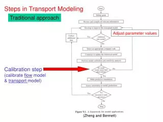
Calibration step (calibrate flow model & transport model). Steps in Transport Modeling. Traditional approach. Adjust parameter values. (Zheng and Bennett). Comparison of measured and simulated concentrations. Average calibration errors (residuals) are reported as:.

E N D
Calibration step (calibrate flow model & transport model) Steps in Transport Modeling Traditional approach Adjust parameter values (Zheng and Bennett)
Comparison of measured and simulated concentrations
Average calibration errors (residuals) are reported as: Mean Absolute Error (MAE) = 1/N calculatedi – observedi Root Mean Squared Error (RMS) = 1/N (calculatedi – observedi)2½ Sum of squared residuals = (calculatedi – observedi)2 Minimize errors; Minimize the objective function
Calibration step (calibrate flow model & transport model) Steps in Transport Modeling Traditional approach Adjust parameter values (Zheng and Bennett)
Input Parameters for Transport Simulation Flow hydraulic conductivity (Kx, Ky Kz) storage coefficient (Ss, S, Sy) recharge rate pumping rates All of these parameters potentially could be estimated during calibration. That is, they are potentially calibration parameters. Transport porosity () dispersivity (L, TH, TV) retardation factor or distribution coefficient 1st order decay coefficient or half life source term (mass flux)
Calibration step (calibrate flow model & transport model) Steps in Transport Modeling Traditional approach Adjust parameter values (Zheng and Bennett)
In a traditional sensitivity analysis, sensitive parameters are varied within some range of the calibrated value. The model is run using these extreme values of the sensitive parameter while holding the other parameters constant at their calibrated values. The effect of variation (uncertainty) in the sensitive parameter on model results Is evaluated. A sensitivity analysis is meant to address uncertainty in parameter values. Problems with this approach: The model goes out of calibration. The results of the sensitivity runs represent unreasonable scenarios.
Dr. John Doherty Watermark Numerical Computing, Australia PEST Parameter ESTimation
New Book 2007 Mary C. Hill Claire R. Tiedeman USGS Modelers
Multi-model Analysis (MMA) Predictions and sensitivity analysis are now inside the calibration loop From Hill and Tiedeman 2007
Input files Input files PEST Model calibration conditions Model predictive conditions Output files Output files Maximise or minimise key prediction while keeping model calibrated
Estimated parameter values; nonlinear case:- p2 Objective function minimum p1
Objective function contours – nonlinear model Likely parameter values p2 p1
Calibration of a flow model is relatively straightforward: • Match model results to an observed steady state flow field • If possible, verify with a transient calibration • Calibration to flow is non-unique. • Calibration of a transport model is more difficult: • There are more potential calibration parameters • There is greater potential for numerical error in the solution • The measured concentration data needed for calibration • may be sparse or non-existent • Transport calibrations are non-unique.
Simulated: smooth source concentration (best calibration) Simulated: double-peaked source concentration (best calibration) Borden Plume Calibration is non-unique. Two sets of parameter values give equally good matches to the observed plume. Z&B, Ch. 14
R=1 R=3 observed R=6 Assumed source input function “Trial and error” method of calibration
Case Study: Woburn, Massachusetts Modeling done by Maura Metheny for the PhD under the direction of Prof. Scott Bair, Ohio State University TCE (Trichloroethene)
0 1000 feet Woburn Site TCE in 1985 Geology: buried river valley of glacial outwash and ice contact deposits overlying fractured bedrock Aberjona River W.R. Grace Municipal Wells G & H Wells G&H operated from October 1964- May 1979 Beatrice Foods The trial took place in 1986. Did TCE reach the wells before May 1979?
Five sources of TCE were included in the model: • New England Plastics • Wildwood Conservation Trust (Riley Tannery/Beatrice Foods) • Olympia Nominee Trust (Hemingway Trucking) • UniFirst • W.R. Grace (Cryovac) Woburn Model: Design MODFLOW, MT3D, and GWV 6 layers, 93 rows, 107 columns (30,111 active cells) Simulation from Jan. 1960 to Dec. 1985 using 55 stress periods (to account for changes in pumping and recharge owing to changes in precipitation and land use) Wells operated from October 1964- May 1979 The transport model typically took two to three days to run on a 1.8 gigahertz PC with 1024K MB RAM.
Calibration of a flow model is generally straightforward: • Match model results to an observed steady state flow field • If possible, verify with a transient calibration • Calibration to flow is non-unique. Calibration Targets: Heads and fluxes • Calibration of a transport model is more difficult: • There are more potential calibration parameters • There is greater potential for numerical error in the solution • The measured concentration data needed for calibration • may be sparse or non-existent • Transport calibrations are non-unique. Calibration Targets: concentrations
Source term input function Used as a calibration parameter in the Woburn model Other possible calibration parameters include: K, recharge, boundary conditions dispersivities chemical reaction terms From Zheng and Bennett
Woburn Model: Trial & Error Calibration • Flow model (included heterogeneity in K, S and ) • Water levels • Streamflow measurements • Groundwater velocities from helium/tritium groundwater ages Transport Model(included retardation) The animation represents one of several equally plausible simulations of TCE transport based on estimates of source locations, source concentrations, release times, and retardation. The group of plausible scenarios was developed because the exact nature of the TCE sources is not precisely known. It cannot be determined which, if any, of the plausible scenarios actually represents what occurred in the groundwater flow system during this period, even though each of the plausible scenarios closely reproducedmeasured values of TCE.
Steps in Modeling Calibration step: calibrate flow model & transport model New Paradigm Traditional approach
“Automated” Calibration Case Study Codes: UCODE, PEST, MODFLOWP From Zheng and Bennett
source term recharge Sum of squared residuals = (calculatedi – observedi)2 Transport data are useful in calibrating a flow model From Zheng and Bennett
Comparison of observed vs. simulated concentrations at 3 wells for the 10 parameter simulation. From Zheng and Bennett